 This tutorial walks you through building and using the Ampere Porting Advisor and how to mitigate any issues.
Continue reading
The Ampere Porting Advisor Tutorial
on SitePoint.
This tutorial walks you through building and using the Ampere Porting Advisor and how to mitigate any issues.
Continue reading
The Ampere Porting Advisor Tutorial
on SitePoint.
 Unlock the best practices for building scalable React apps. Explore strategies for performance, maintainability, state management, code splitting, and real-world success stories.
Continue reading
How to Build Scalable Web Apps with React JS
on SitePoint.
Unlock the best practices for building scalable React apps. Explore strategies for performance, maintainability, state management, code splitting, and real-world success stories.
Continue reading
How to Build Scalable Web Apps with React JS
on SitePoint.
今天我将介绍一下怎么用 AI + 自动化工具,实现播客内容的“一次制作、多平台分发”。
播客是啥?现在谁还在听?
播客(英文:Podcast)是指的是通过数字广播技术制作的,在互联网上传播的音频内容。简单来说,播客就是“可以订阅的音频节目”,你可以把它理解成“音频版的专栏文章”或者“随时能听的电台节目”。它不像直播那样需要你盯着屏幕,也不像视频那样吃流量,适合开车、做饭、散步的时候听。
在内容泛滥的今天,播客反而成了注意力稀缺下的“净土”——节奏慢、干货多、听众粘性强。
目前主流播客平台包括:
国内平台: 喜马拉雅、网易云音乐、小宇宙
海外平台: Apple Podcasts、Spotify、YouTube Music、Pocket Casts
大部分平台都支持用 RSS Feed 自动订阅内容更新——这就是我们可以“自动同步”的关键点。
根据《PodFest China2020中文播客听众与消费调研》显示,中文播客听众最常使用的5个收听渠道是:Apple Podcasts(49.7%)、喜马拉雅(37.9%)、网易云音乐 (35.0%)、微信公众号内嵌音频 (21.9%)和Pocket Casts(19.5%)。

为什么要自动更新播客?
我们做内容的都知道,最大的问题不仅仅是创作,而且发布太繁琐也是个大问题。你要一条条上传音频、写描述、同步封面,光是把一集播客发到5个平台,就能让人劝退。
但如果有个方法,可以让我只上传一次,就能全平台同步更新,是不是省时省力又体面?于是就有了这套玩法:AI生成播客 + 多平台同步。
第一步:用AI批量生成播客内容
先说最核心的一步——播客内容从哪来?
我的方法是:找一些结构化或主题清晰的素材(比如电子书章节、技术文章合集、行业报告等),然后分批导入 NotebookLM 这个工具。
这个工具的牛点在于,它能理解资料内容,然后你可以通过提示词让它生成一段质量不错的,类似播客主持人口吻的音频。通过对提示词的调整,可以从不同角度来优化和调整输出的播客音频。
第二步:在主平台创建播客并上传音频
内容搞定之后,得找个“主阵地”上传音频文件。我试了两家:
Spotify for Podcasters(海外)
喜马拉雅(国内)
这两家都有一个共同特点:能生成 RSS Feed,用户量大。
这个 RSS Feed 非常关键,它就像播客的“分发中枢”,有了它,其他平台就可以自动订阅并更新你的播客内容。
这里重点讲一下喜马拉雅的RSS Feed,隐藏的非常深,不容易找到,登录喜马拉雅创作中心后台,点击“创作实验室”,选择“Apple 播客托管服务”,即可生成一个RSS Feed,这个RSS Feed不仅仅可以同步到Apple Podcasts,同步到其他播客平台也没问题。
Spotify的RSS Feed就好找多了,登录spotify for creators的后台,点击“设置”-“Availability”,即可看到RSS Distribution里面的链接。
你上传好音频,设置好标题、描述、封面,播客就上线了,同时也自动生成了对应的 RSS 链接。
第三步:把RSS同步到其他平台
拿着刚才生成的 RSS 链接,我们可以去以下平台注册并导入:iTunes Podcasts(Apple)、YouTube Music、网易云音乐、小宇宙、Pocket Casts等等。
这些平台在创建播客时一般都有“使用RSS导入”选项,只要粘贴你的链接,它们就能自动抓取更新。
这样一来,你只需要维护喜马拉雅或者Spotify的那一个源头,其余平台会自动同步更新,不用你操心。
后续更新流程就是“一次上传,全网同步”。
从第二期音频开始,你就爽了。流程如下:
把新内容丢进 NotebookLM,设计一个提示词,生成音频。
上传音频到你的主平台(比如喜马拉雅)。
所有绑定RSS的平台都会自动更新。
这不就是我们程序员最爱的“自动化工作流”吗?
一些实用小贴士
素材限制: NotebookLM 对处理的文本长度(包括中文)有以下限制:1、按来源文件限制:每个上传到 NotebookLM 的来源文件(例如 PDF、Google 文档、文本文件等)的字数上限为 50 万字。同时,上传的本地文件大小上限为 200MB。2、按笔记本限制:一个笔记本中可以包含的来源数量,普通用户上限为 50个。
节奏控制: AI生成内容最好控制在10~20分钟,既不累也容易被听完。
配图和封面: ChatGPT出图非常快,图片质量高,顺手还能给社媒配套宣传图。
结语:别等完美,先上车
很多人总觉得做播客门槛高,其实现在有了AI工具和自动化同步工具,真的不难。重要的不是一开始多完美,而是先跑起来,优化可以慢慢来。
如果你也想做知识型播客,这套方法值得一试:轻量、自动化、省心、可扩展。
我的播客地址
下面是我自己创建的各个平台的播客地址:
YouTube:https://www.youtube.com/@williamlong
Apple Podcasts:https://podcasts.apple.com/podcast/%E6%9C%88%E5%85%89%E6%92%AD%E5%AE%A2/id1816103541
Spotify:https://open.spotify.com/show/5L8RZKHcSwfLFzC1qFNNs6
喜马拉雅:https://www.ximalaya.com/album/92461056
网易云音乐:https://music.163.com/#/djradio?id=1224404483
小宇宙:https://www.xiaoyuzhoufm.com/podcast/68302549457b22ce0d25dc08
记得第一季结尾那个令人窒息的时刻吗?火萤组织准备用艾莉的大脑做实验寻找疫苗,实验的过程将杀死艾莉,而乔尔选择大开杀戒救出艾莉,乔尔的行为到底是不是自私让人争论不休,而我,完全理解乔尔的每一个选择。
火萤的行为简直可以写入医学伦理学反面教材。他们对待艾莉的方式,就像对待一个装着解药的容器,而非一个有思想有感情的人。这让我想起康德那句著名的话:"人应该作为目的本身而存在,而不仅仅是手段",火萤恰恰把艾莉当成了手段——一个可能拯救人类的手段。他们甚至懒得询问这个15岁女孩的意愿,就直接准备开颅手术。这种"杀死一个人,拯救千万人"的极端功利主义逻辑,在哲学课本上恐怕都难以自圆其说。
道德的底线是对人的尊重,火萤通过手术杀死艾莉的行为,艾莉完全不知情,也没有做出选择,糊里糊涂就被麻醉上了手术室,火萤如果事先争取艾莉的意见,艾莉同意牺牲自己的生命,那么火萤再做手术,至少符合程序上的合法性。但从剧情上看,即使艾莉不同意手术,火萤也会强行做手术。
强迫一个人牺牲自己来拯救其他人,即不道德,也不合法。火萤的行为符合"牺牲少数拯救多数"的功利主义逻辑,但忽视了个体权利的绝对性。
乔尔不能帮助艾莉做选择,选择她是否牺牲,乔尔去拯救艾莉,维护了艾莉做为一个人最基本的个体权利:生命权,这才是符合最基本的伦理学的道德标准,乔尔将艾莉视为女儿,保护家人的义务高于针对陌生人的义务,乔尔得知火萤计划立即对艾莉进行致命手术(未经其知情同意),且时间紧迫,火萤士兵也试图阻止乔尔,并直接开枪攻击,乔尔随时存在生命危险,因此,在拯救艾莉过程中乔尔杀死全副武装的火萤士兵,是完全必要的,并且不存在任何道德上的问题,在手术室里,主治医生手持手术刀(可算为致命武器)进行阻挡,乔尔杀死医生的行为略有一点点不妥,算是超微超出了一点必要限度,实际上将医生击伤即可。
总的来说,艾莉的险情源于火萤的决定(未经同意进行手术),而非乔尔的过错,乔尔的行大部分为符合紧急避险的规则。
不过,乔尔最后杀死马琳的行为存在较大争议,主要动机是为了确保火萤不会追杀,属于乔尔人性的黑暗面,但鉴于马琳是制造险情的元凶,因此简单判断对错也是非常困难的。
第二季最精彩的地方在于它没有简单地评判对错,艾比的故事线让观众被迫站在"另一边"思考:如果你的父亲是被乔尔杀死的医生,你会怎么做?这种视角转换简直是对观众道德观的一次"压力测试",尼采说"当你凝视深渊时,深渊也在凝视着你",这部剧完美诠释了这句话——我们越是深入每个角色的动机,就越难做出简单的道德判断。
特别打动我的是艾莉和乔尔之间逐渐修复的关系,那些安静的瞬间——一起弹吉他、看长颈鹿、讲蹩脚笑话——比任何枪战戏都更有力量,在这个道德模糊的世界里,他们之间的爱是少数几件确定无疑的美好事物。这让我想起自己和子女的关系:青春期时我们吵得天翻地覆,但子女大学毕业了,我们反而能像朋友一样相处。人类关系的韧性,或许才是对抗这个荒谬世界的最佳武器。
《最后生还者》第二季最伟大的地方在于,它拒绝给出简单答案。在这个后末日世界里,每个人都在为自己的生存和所爱之人战斗,每个人的选择都有其合理性,但又都沾满鲜血。萨特说"他人即地狱",但这部剧告诉我们:没有他人,我们也终将成为自己的地狱。当乔尔抱着受伤的艾莉穿过医院走廊时,他选择了一个具体的人而非抽象的人类——而这,或许就是混乱世界中我们能做的最人性的选择。
 最近的一個架站需求,案主需要翻譯網站文字的功能,點擊指定按鈕後,自動將網頁上的中文轉換為英文。這樣的作法,比起另外製作英文版網站,可省下不少成本與時間。
十多年前曾寫過「讓 Google 網頁翻譯工具以國旗超連結執行」,該篇的作法是點擊國旗連結後,另開頁面呈現翻譯效果,無法在同頁面直接翻譯。這麼多年過去了,想必可以有更好的作法。
經研究後,Blogger 網站很容易就能作到這件事,因為後台官方就提供了「翻譯」小工具,可直接安裝在往站上。本篇會說明如何利用這個小工具,經由自製的國旗圖示,點擊後立即將網頁內容翻譯成對應的語言。
最近的一個架站需求,案主需要翻譯網站文字的功能,點擊指定按鈕後,自動將網頁上的中文轉換為英文。這樣的作法,比起另外製作英文版網站,可省下不少成本與時間。
十多年前曾寫過「讓 Google 網頁翻譯工具以國旗超連結執行」,該篇的作法是點擊國旗連結後,另開頁面呈現翻譯效果,無法在同頁面直接翻譯。這麼多年過去了,想必可以有更好的作法。
經研究後,Blogger 網站很容易就能作到這件事,因為後台官方就提供了「翻譯」小工具,可直接安裝在往站上。本篇會說明如何利用這個小工具,經由自製的國旗圖示,點擊後立即將網頁內容翻譯成對應的語言。


一、用 JS 執行翻譯的原理
1. Google 翻譯工具的缺點 Google 翻譯工具使用久了就會覺得麻煩,每次都得從下拉選單中找出想使用的語言,而偏偏選項密密麻麻,得浪費不少時間。 所以對於訪客比較友善的設計會是,將幾種常用的語言獨立出來,例如做成國旗圖案按鈕,放在頁面上顯眼之處,點擊後立即看到效果,可省下訪客不少時間。 為了實現這個目標,我們得找出能夠直接用 JS 執行翻譯的指令為何。 2. 用 JS 執行翻譯 Google 搜尋的結果,我找到這兩篇很有參考價值: 簡單說一下原理,方法是利用 JS 操作 Google 翻譯的下拉選單,模擬選取想要的語言後,觸發選單的切換選項動作,讓 Google 翻譯工具自動執行該選項。 3. 找出語言對應的參數 接下來,JS 執行時會用到的語言參數,可參考 Google 翻譯官網「Language support」,以下順便列出常用的翻譯語言參數:- 英文:en
- 簡中:zh-CN
- 日文:ja
- 韓文:ko
- 法文:fr
- 西班牙:es
二、安裝 Google 翻譯工具
1. Blogger 網站 如果是 Blogger 網站的話比較輕鬆一些,安裝 Blogger 官方提供的翻譯小工具步驟如下:- 後台 → 版面配置 → 新增小工具 → 翻譯
- 安裝完後,編輯這個小工具,「樣式」可以選擇「縱向」,但切記不可選擇「僅限下拉式選單」,這非常重要!
<div id="google_translate_element"></div>
<script>
	function googleTranslateElementInit() {
		new google.translate.TranslateElement({
			pageLanguage: "zh-TW",
			autoDisplay: false,
			layout: google.translate.TranslateElement.InlineLayout.VERTICAL
		}, "google_translate_element");
	}
</script>
<script src="//translate.google.com/translate_a/element.js?cb=googleTranslateElementInit"></script>
三、安裝程式碼
1. 準備動作 在修改範本之前,如果第一次安裝本站工具的讀者,建議先閱讀「備份範本的訣竅」系列文章。 請到後台「主題」→ "自訂" 按鈕右方的下拉圖示 →「編輯 HTML」,游標點進範本區塊,按 Ctrl-F 搜尋<script src='//ajax.googleapis.com/ajax/libs/jquery/2.0.0/jquery.min.js'></script>
可參考「引用 jQuery 的注意事項」,檢查範本是否已安裝過 jQuery,如果已經安裝過請刪除此行,以免重複安裝。
2. 安裝程式碼
國旗按鈕想要放在網站什麼地方,可參考「Blogger 範本各區塊程式碼」,找到自己想擺放的位置。
在後台「主題」→ "自訂" 按鈕右方的下拉圖示 →「編輯 HTML」,游標點進範本區塊,找到你想放的位置後,貼上以下程式碼:
<!--國旗翻譯工具-->
<div id="flag_translate">
	<img class="en" src="https://3.bp.blogspot.com/-lPe1MfSK7zs/UXaYYpJ-lJI/AAAAAAAAGiU/FIBrY3aIhW0/s1600/eng.jpg" alt="英文">
	<img class="zh-CN" src="https://4.bp.blogspot.com/-HqR8f67uo9g/UXaVG1JlVEI/AAAAAAAAGhs/9Ak-hJ-UGRA/s1600/cn.jpg" alt="簡中">
	<img class="ja" src="https://1.bp.blogspot.com/-kCzI3AnvG1c/UXaYZZ7IBDI/AAAAAAAAGic/bt6V0kD-Ong/s1600/jp.jpg" alt="日文">
</div>
<style>
	#flag_translate img{margin-right: 10px; cursor: pointer;}
</style>
<script>
	//<![CDATA[
	$("#flag_translate img").click(function() {
		let className = this.className;
		let $select = $("#google_translate_element select");
		$select.val(className);
		setTimeout(function() {
			$select[0].dispatchEvent(new Event("change"));
		}, 10);
	});
	//]]>
</script>
<!--Designed by WFU BLOG-->
儲存後即可看到效果。
3. 修改參數
想要自訂參數、圖案的話,請見以下說明:
- 紅字參數:請參考「一、用 JS 執行翻譯的原理」→「3. 找出語言對應的參數」來修改
- 藍字參數:請改為自己的國旗圖案網址
四、補充+展示效果
- 上面三個國旗按鈕,可點擊後看翻譯效果
- 由於不需要操作「翻譯」小工具,那麼側邊欄的這個小工具,也可用 CSS 自行隱藏起來
本杂志开源,欢迎投稿。另有《谁在招人》服务,发布程序员招聘信息。合作请邮件联系(yifeng.ruan@gmail.com)。
封面图

北京的护城河公共绿道,位于鼓楼附近。(via visuals_china@instagram)
神经网络算法的发明者
上周的《李飞飞自传》读后感,还有后续。那篇文章的结尾是,2012年一支加拿大团队使用神经网络算法,夺得了 ImageNet 比赛冠军。
今天就来说说,这支加拿大团队的故事。

大家看了就知道了,神经网络算法是怎么诞生的,背后的推手又是谁。
(1)杰弗里·辛顿(Geoffrey Hinton,1947-)

辛顿出生于英国,后移居加拿大。他是神经网络算法的奠基人和主要发明者。
神经网络的概念,是上世纪40年代后期提出的(提出人不是辛顿)。当时的想法是,既然人类通过神经网络进行思考,那么只要让机器模拟神经网络,机器就能思考了。
但是,那只是一个概念,并没有具体的算法。机器怎么模拟思考,人们并不知道。
1984年,辛顿在加州大学担任博士后,与两个同事一起提出了反向传播算法。
这个算法可以建立多层网络,产生一个输出结果,让神经网络变成了现实,也是后来更高级算法的基础。
由于它需要多层计算,后一层在前一层的结果上学习,所以被称为"深度学习",辛顿因此成为"深度学习之父"。
辛顿后来因为这个贡献,获得了图灵奖(2018年)和诺贝尔物理学奖(2024年)。
(2)杨立昆(1960-)

杨·安德烈·勒坎(Yann André Le Cun,中文名杨立昆)是法国人。上个世纪80年代,他是多伦多大学博士后。
这一时期,辛顿也来到了多伦多大学任教,担任他的指导教师。
所以,杨立昆是辛顿的大弟子,继承和发展了辛顿的算法。他的主要成就是,为神经网络引入了卷积算法,并且做出了第一个有实际用途的神经网络。
1990年代,他用神经网络识别银行支票的手写数字,成功获得了企业的采用。

但是,这个应用也暴露了卷积神经网络的弱点:它需要大量样本的训练,耗费巨大的算力。银行支票只需要识别10个阿拉伯数字,如果是更多样化的场景,当时的计算能力难以做到。
学术界因此认为,卷积神经网络只适用特定的、计算量较小的场景,不具备推广的价值。这导致这种算法,以及辛顿和杨立昆,被冷落了二十年。
这二十年,杨立昆一直混迹于企业实验室和大学教研室。等到世界重新认识卷积神经网络,他在2018年与辛顿一起获得了图灵奖,现在是 Meta 公司的副总裁和 AI 首席科学家。
(3)亚历克斯·克里泽夫斯基(Alex Krizhevsky,1986-)

亚历克斯·克里泽夫斯基是乌克兰人,少年时随家人移民到加拿大。2007年,他进入多伦多大学,成为辛顿的博士生。
这时距离杨立昆提出卷积神经网络,已经过去快20年了。辛顿始终没忘记它,他鼓励亚历克斯和稍后要提到的伊尔亚·苏茨克维,使用这种算法,去挑战李飞飞的 ImageNet。
亚历克斯就写了一个程序,用 ImageNet 的1500万图片,来训练他的卷积神经网络。但是,计算量太大了,他的个人计算机根本跑不动,他就买了两块 Nvidia 显卡,每天24小时一刻不停地运算。
事实证明,卷积神经网络+大训练集+高速计算硬件,超过了其他一切已知的算法。最终,他们的三人团队以巨大优势,夺得了2012年第三届 ImageNet 算法比赛冠军。
这件事轰动了业界,各大互联网公司纷纷邀请辛顿和他的学生加入。百度也伸出橄榄枝,邀请辛顿担任首席科学家,但是最后输给了谷歌。
2013年,谷歌以4400万美元收购了辛顿成立的空壳公司,将辛顿、亚历克斯、伊尔亚三个人一起招入麾下。
2017年,亚历克斯辞职,现在一家创业公司研究 AI 技术。
(4)伊尔亚·苏茨克维(Ilya Sutskever, 1986-)

伊尔亚·苏茨克维出生于前苏联,后去了以色列,然后来到加拿大。他是亚历克斯·克里泽夫斯基在多伦多大学的博士同学,也是辛顿的博士生。
他与亚历克斯组成团队,共同赢得了2012年的 ImageNet 算法比赛。辛顿作为指导老师,也是团队一员。
他在2013年跟随辛顿加入谷歌,2015年辞职,成为 OpenAI 的联合创始人和首席科学家,后来是 ChatGPT 的主要作者之一。2024年,他离开 OpenAI,现在创立了自己的 AI 公司。
(5)安德烈·卡帕斯(Andrej Karpathy,1986-)

安德烈·卡帕斯出生于斯洛伐克,15岁随家人来到加拿大,在多伦多大学读完了本科。
他跟伊尔亚·苏茨克维很可能大学里就认识。但是,他没在多伦多大学读博士,而是去了斯坦福大学,指导老师就是李飞飞。
他的方向也是卷积神经网络,博士期间开设了斯坦福大学第一门深度学习课程,担任主讲。
2015年,他跟随伊尔亚一起加入 OpenAI,成为主要研究人员。
2017年,他离开 OpenAI,去了特斯拉,担任特斯拉 AI 总监,2022年离职。
(6) 总结
上面五人是神经网络算法的主要创立者和推动者。没有他们,就不会有今天的 AI 大模型。
但是,单单靠他们的算法,AI 不会成功。因为算法需要大量的数据进行训练,而训练需要高速计算的硬件。这三者缺一不可。
只有等到2012年,才万事俱备。神经网络算法 + 李飞飞的 ImageNet 训练集 + Nvidia 高速显卡,同时出现了。
历史于是翻开了新的一页,AI 时代正式来临。
科技动态
(1)一家深圳公司推出了,可能最炫酷的树莓派机箱。
它自带机箱显示屏、RGB 灯光、风扇、NVMe SSD 扩展板,很适合用作 NAS 和 AI 边缘计算。

(2)芬兰尝试在驯鹿的鹿角,涂上荧光粉。

这是为了方便司机在夜间看到驯鹿,目前每年在芬兰公路上被撞死的驯鹿有4000头。
(3)在线会议软件 Google Meet,推出实时语音翻译,首先提供西班牙语版本。

在线会议时,对方说西班牙语,你听到的却是英语,而且声音、语调和情感都不变。
(4)意大利开源硬件公司 Arduino,研发出了可降解 PCB(电路板),减轻对环境的污染。

这种可降解电路板,将电路印刷在植物亚麻材料上,而不是传统的玻璃纤维和树脂。
不过,电路板上的铜无法降解,需要在丢弃电路板之前先回收。
(5)一家美国创业公司,准备发射卫星,将 AI 机房建在太空。

它依靠24小时的太阳能供电,也不用担心散热。
该公司希望通过这种方法,解决 AI 服务器的耗电和冷却问题。
文章
1、手机的 Linux 桌面环境(英文)作者出门不带笔记本,只带手机,再配上蓝牙键盘和 AR 眼镜。

他的安卓手机在获取 root 权限后,通过 chroot 安装了 Linux 发行版,从而可以运行桌面环境。

2、AI 应用的核心逻辑(英文)

作者提出,AI 应用(AI agent)的核心逻辑只需要9行代码。
3、浏览器默认屏蔽的端口(英文)

你可能不知道,浏览器无法打开下面的网址
localhost:6000,原因是6000是浏览器默认屏蔽的端口。4、推荐 RustDesk 远程桌面(英文)

Mac 电脑访问 Windows 电脑,一种方法就是使用远程桌面,作者推荐远程桌面工具 RustDesk。
5、HTML
<dialog> 的 CSS 技巧(英文)
HTML 有一个原生的弹窗元素
<dialog>,本文介绍两个配套使用的 CSS 技巧。6、Git 配置详解(英文)

本文详细解释 Git 配置命令 git config 的几个最常见的设置。
工具
1、Pyrefly
Meta 公司发布的 Python 代码的类型检查器,参见介绍文章。
2、Zen Browser

新发布的一个开源浏览器,基于 Firefox,国外评价非常高,使用体验好,参见介绍文章。
3、xtool

Xcode 的替代品,在 Linux/Win/macOS 开发 iOS 应用。
4、Zero Convert

在线批量转换文件,基于 WebAssembly 技术,完全本地完成,还可以编辑图片。(@xiaoshangmin 投稿)
5、耗子面板

Go 语言开发的服务器管理面板。(@devhaozi 投稿)
6、Goravel

Go 语言的 Web 开发框架,与 PHP 的 Laravel 框架保持一致,方便快速上手。(@devhaozi 投稿)
7、OpenSpeedy
开源的游戏变速工具,通过调整 Windows 系统时间函数来实现游戏速度变化。(@game1024 投稿)
8、SimonAKing-Gallery

后端的 JS 相册应用,瀑布流展示图片,指定图片目录,直接运行即可。(@SimonAKing 投稿)
9、Jwno

网友开源的 Windows 10/11 平铺窗口管理器,键盘驱动。(@agent-kilo 投稿)
10、星河小程序

滴滴公司开源的跨平台开发框架,支持将小程序打包成为安卓、iOS、鸿蒙和 Web 四个平台的原生 App。(@dos1in 投稿)
AI 相关
1、aTrain
一个跨平台、图形界面的自动语音识别工具,基于 Whisper 模型,支持识别50多种语言,参见介绍文章。
2、AI Image Editor

在线的免费图像处理工具,提供多种 AI 功能,比如图片增强、去除水印、风格转换等十几种。(@worminone 投稿)
资源
1、万物博物馆一个跨平台的桌面软件,将维基百科变成一个虚拟博物馆。

每件展品与维基百科的一篇文章相对应,墙上的画框就是文章图片,讲解牌就是文章内容。

走廊则根据文章的链接通向其他展厅,有几乎无限的展厅可以参观。

图片
1、《星球大战》的机器人《星球大战》的第一部电影,拍摄于1976年,里面有一个机器人 R2-D2,会四处走动,做各种动作,还会说话。

其实,它根本没那么高科技,拍摄的时候,就是里面藏了一个真人演员。

2、冰为什么体积大?
水变成冰以后,体积会增大10%,密度因此小于水,使得冰可以浮在水面上。
那么,冰的体积为什么会增大呢?
答案是冰的分子结构,跟水的分子结构不一样。

上图左侧是液态水的分子结构,右侧是冰的分子结构。其中,白色节点为氢原子,红色节点为氧原子。
可以看到,液态水是紧密聚合的网络结构,冰则是中空的网络结构。也就是说,冰的分子结构不是那么密合,所以体积就变大了。
文摘
1、Slack 公司的 URLSlack 是一家即时通信的软件公司。它的官网有一个"公司介绍"的页面,通常来说该页面的 URL 会是
slack.com/about,但是 Slack 没有采用这种做法。它将这个页面命名为
is,并分拆成若干个子页面。所以,"公司介绍"页面的 URL 是
slack.com/is。子页面的 URL 如下。
- slack.com/is/team-communication
- slack.com/is/everything-in-one-place
- slack.com/is/wherever-you-are
这样的好处是单单看 URL,就知道页面想要传递的信息,URL 本身就是对公司的一种宣传。
这种 is 的巧妙做法,后来被广泛借鉴。碰巧的是,
is也正好是一个顶级域名,代表冰岛(iceland)。很多名人就申请了 is 域名,作为个人主页。比如,艺术家杰西卡·希斯切(Jessica Hische)的个人网站,域名就是
jessicahische.is,她介绍自己的页面 URL 就都是jessicahische.is/xxx的形式。言论
1、我们很快会跟大家分享一个低调的研究成果。我们会给它起一个比 chatGPT 更好的名字,以防它流行起来。
-- Sam Altman,OpenAI 的 CEO
2、
加尔定律经常被引用:"一个有效的复杂系统,总是从一个有效的简单系统进化而来。"
但是,它的推论很少被引用:"一个从零开始设计的复杂系统永远不会有效,你必须从一个可以运行的简单系统开始。"
-- Stack Staves
3、
宇宙有两种可能:要么我们是孤独的,要么我们并不孤独。这两种可能性都同样令人恐惧。
-- 阿瑟·克拉克,英国著名科幻小说家
4、
太阳绕银河系公转一圈需要2.3亿年,上一圈的时候,地球的主宰还是恐龙。
-- Reddit 网友
5、
我关注了一些教育工作者,他们都报告了同样的现象:他们的学生什么事情都用 ChatGPT,结果什么也没学到。
最终可能会出现这样一代人,自己的智力很低下,完全依赖于他们不理解的技术,一旦技术崩溃,他们永远无法从头开始重建。
-- 尼尔·斯蒂芬森(Neal Stephenson),美国科幻小说家,"元宇宙"一词的创造者
往年回顾
创业虽然好,不敢推荐了(#302)互联网创业变难了(#252)
三个有启发的学习方法(#202)
从北大到技校(#152)
(完)
文档信息
- 版权声明:自由转载-非商用-非衍生-保持署名(创意共享3.0许可证)
- 发表日期: 2025年5月23日
The post Agent mode 101: All about GitHub Copilot’s powerful mode appeared first on The GitHub Blog.
The post Shine a spotlight on your open source project appeared first on The GitHub Blog.
The post Bypassing MTE with CVE-2025-0072 appeared first on The GitHub Blog.
The post Announcing TypeScript Native Previews appeared first on TypeScript.
Since this release, there has been a constant question from the AI community: could an open-source VLM be an image generator as capable as GPT-4o? We’ve covered this topic on the DigitalOcean Tutorials blog with Janus Pro, but that model was decidedly too small to match the likes of even Stable Diffusion 1.5 at image generation tasks, despite its reportedly higher ELO.
This week, the question may have been answered with ByteDance SEED’s newest release: the BAGEL model. This first-of-its-kind, massive open-source VLM is the largest vision language model ever released to the public, and it shows impressive results already. With 14B (7B active) parameters, it is one of the largest models of it’s kind. Not only can it describe images with details akin to some of the best closed-source models, it can even generate and edit images to a high degree of accuracy. This is all thanks to their unique mixture-of-transformers-experts (MoT) that selectively activates modality specific parameters to optimize the results. For more information about how BAGEL works, check out their paper.
In this tutorial, we will show how to run BAGEL on a GPU Droplet using the provided Jupyter Notebook based examples from the project’s repository on Github. Follow along for instructions on setting up a GPU Droplet to run BAGEL followed by detailed explanations of the model’s capabilities in practice.
Running BAGEL on DigitalOcean’s GPU Droplets
In this section of the tutorial, we will show how to set up the environment for BAGEL on a GPU Droplet, and then show some examples of images we generated using the code provided.Set Up the GPU Droplet for BAGEL
To get started, sign into your DigitalOcean account and spin up an NVIDIA GPU powered GPU Droplet. We recommend either a single or eight way NVIDIA H100 GPU Droplet for running this model. Follow the instructions in this article to set up your environment for this tutorial, as we will need to have added our SSH keys to the GPU Droplet and installed Jupyter to continue.Once your GPU Droplet is running, we can SSH into our GPU Droplet from our local machine’s terminal. To set up the environment for this demo, paste the following code into your terminal:
apt install python3-pip python3.10-venv
pip install huggingface-hub wheel jupyter
git clone https://github.com/ByteDance-Seed/Bagel
cd Bagel/
vim requirements.txt
flash_attn==2.5.8 from the text file. This will prevent a broken install later on. Alternatively, you can directly remove it by accessing the host machine from your local VS Code application, and using the file editor to modify the text file. Once that’s done, we can continue with installation.pip install -r requirements.txt
pip install git+https://github.com/Dao-AILab/flash-attention
huggingface-cli login

##After entering your access token

huggingface-cli download ByteDance-Seed/BAGEL-7B-MoT --local-folder ./BAGEL-7B-MoT
from huggingface_hub import snapshot_download

save_dir = "./BAGEL-7B-MoT"
repo_id = "ByteDance-Seed/BAGEL-7B-MoT"
cache_dir = save_dir + "/cache"

snapshot_download(cache_dir=cache_dir,
        local_dir=save_dir,
        repo_id=repo_id,
        local_dir_use_symlinks=False,
        resume_download=True,
        allow_patterns=["*.json", "*.safetensors", "*.bin", "*.py", "*.md", "*.txt"],
        )
jupyter lab --allow-root
Then copy the URL output, and use that to paste into the simple browser in your VS Code window as shown in the setup tutorial.
Now that we have accessed our Jupyter Lab environment on our local browser, let’s get started with BAGEL. Open the
inference.ipynb notebook file, and run the first 7 code cells. These are labeled to correspond to what each does for the setup process.import os
from copy import deepcopy
from typing import (
Any,
AsyncIterable,
Callable,
Dict,
Generator,
List,
NamedTuple,
Optional,
Tuple,
Union,
)
import requests
from io import BytesIO
from PIL import Image
import torch
from accelerate import infer_auto_device_map, load_checkpoint_and_dispatch, init_empty_weights
from data.transforms import ImageTransform
from data.data_utils import pil_img2rgb, add_special_tokens
from modeling.bagel import (
BagelConfig, Bagel, Qwen2Config, Qwen2ForCausalLM, SiglipVisionConfig, SiglipVisionModel
)
from modeling.qwen2 import Qwen2Tokenizer
from modeling.bagel.qwen2_navit import NaiveCache
from modeling.autoencoder import load_ae
from safetensors.torch import load_file
./BAGEL-7B-MoT.model_path = "./BAGEL-7B-MoT"
# LLM config preparing
llm_config = Qwen2Config.from_json_file(os.path.join(model_path, "llm_config.json"))
llm_config.qk_norm = True
llm_config.tie_word_embeddings = False
llm_config.layer_module = "Qwen2MoTDecoderLayer"
# ViT config preparing
vit_config = SiglipVisionConfig.from_json_file(os.path.join(model_path, "vit_config.json"))
vit_config.rope = False
vit_config.num_hidden_layers = vit_config.num_hidden_layers - 1
# VAE loading
vae_model, vae_config = load_ae(local_path=os.path.join(model_path, "ae.safetensors"))
# Bagel config preparing
config = BagelConfig(
visual_gen=True,
visual_und=True,
llm_config=llm_config,
vit_config=vit_config,
vae_config=vae_config,
vit_max_num_patch_per_side=70,
connector_act='gelu_pytorch_tanh',
latent_patch_size=2,
max_latent_size=64,
)
with init_empty_weights():
language_model = Qwen2ForCausalLM(llm_config)
vit_model = SiglipVisionModel(vit_config)
model = Bagel(language_model, vit_model, config)
model.vit_model.vision_model.embeddings.convert_conv2d_to_linear(vit_config, meta=True)
# Tokenizer Preparing
tokenizer = Qwen2Tokenizer.from_pretrained(model_path)
tokenizer, new_token_ids, _ = add_special_tokens(tokenizer)
# Image Transform Preparing
vae_transform = ImageTransform(1024, 512, 16)
vit_transform = ImageTransform(980, 224, 14)
max_mem_per_gpu = "80GiB"  # Modify it according to your GPU setting

device_map = infer_auto_device_map(
    model,
    max_memory={i: max_mem_per_gpu for i in range(torch.cuda.device_count())},
    no_split_module_classes=["Bagel", "Qwen2MoTDecoderLayer"],
)
print(device_map)

same_device_modules = [
    'language_model.model.embed_tokens',
    'time_embedder',
    'latent_pos_embed',
    'vae2llm',
    'llm2vae',
    'connector',
    'vit_pos_embed'
]

if torch.cuda.device_count() == 1:
    first_device = device_map.get(same_device_modules[0], "cuda:0")
    for k in same_device_modules:
        if k in device_map:
            device_map[k] = first_device
        else:
            device_map[k] = "cuda:0"
else:
    first_device = device_map.get(same_device_modules[0])
    for k in same_device_modules:
        if k in device_map:
            device_map[k] = first_device

model = load_checkpoint_and_dispatch(
    model,
    checkpoint=model_path+"/ema.safetensors"),
    device_map=device_map,
    offload_buffers=True,
    dtype=torch.bfloat16,
)

model = model.eval()
print('Model loaded')
from inferencer import InterleaveInferencer

inferencer = InterleaveInferencer(
        model=model,
        vae_model=vae_model,
        tokenizer=tokenizer,
        vae_transform=vae_transform,
        vit_transform=vit_transform,
        new_token_ids=new_token_ids
)

import random
import numpy as np

seed = 42
random.seed(seed)
np.random.seed(seed)
torch.manual_seed(seed)
if torch.cuda.is_available():
        torch.cuda.manual_seed(seed)
        torch.cuda.manual_seed_all(seed)
torch.backends.cudnn.deterministic = True
torch.backends.cudnn.benchmark = False
Generate images with BAGEL
To generate images, navigate to the section of the notebook labeled “Image Generation”. Run the first code cell to instantiate a dictionary with the parameters for the inference run. Then run the following cell to generate your image. Below is an example using the code from both cells:inference_hyper=dict(
cfg_text_scale=4.0,
cfg_img_scale=1.0,
cfg_interval=[0.4, 1.0],
timestep_shift=3.0,
num_timesteps=50,
cfg_renorm_min=1.0,
cfg_renorm_type="global",
)
prompt = '''draw the famous actor Keanu Reeves with long hair and a beard eating Ramen noodles while sitting next to an anthromorphic bear wearing a bowtie, both laughing, drawing in anime style'''
print(prompt)
print('-' * 10)
output_dict = inferencer(text=prompt, **inference_hyper)
display(output_dict['image'])

from PIL import Image
import PIL

output_dict['image'].save('output_img_gen.png')
Generate Images with Thinking
Next, we will take advantage of the VLM’s reasoning capabilities to augment the control of our image generation. In practice, it appears the VLM expands and rewrites the prompt to try and better express the user’s original intent. Below, we can see the code used to generate an image with thinking.inference_hyper=dict(
max_think_token_n=1000,
do_sample=False,
# text_temperature=0.3,
cfg_text_scale=4.0,
cfg_img_scale=1.0,
cfg_interval=[0.4, 1.0],
timestep_shift=3.0,
num_timesteps=50,
cfg_renorm_min=1.0,
cfg_renorm_type="global",
)
prompt = '''draw the famous actor Keanu Reeves with long hair and a beard eating Ramen noodles while sitting next to an anthromorphic bear wearing a bowtie, Keanu is wearing a shirt that says "DigitalOean", both are laughing, drawing in anime style'''
print(prompt)
print('-' * 10)
output_dict = inferencer(text=prompt, think=True, **inference_hyper)
print(output_dict['text'])
display(output_dict['image'])
“”" think Okay, let’s break this down. The user wants an anime-style drawing of Keanu Reeves with long hair and a beard, eating Ramen noodles. He’s sitting next to an anthropomorphic bear wearing a bowtie. Keanu is wearing a shirt that says “DigitalOcean,” and both are laughing. The scene should be vibrant and playful, with a focus on the characters’ expressions and the food. I need to ensure the bear is drawn in a cute, human-like manner, and the shirt text is clearly visible. The overall tone should be light-hearted and fun, with exaggerated anime features like big eyes and dynamic lines. end think “”"
This generated the example image below:

As we can see, the image is fairly similar to the original. We would argue that the quality is a bit higher, with greater prompt adherence, as shown by the more anime-like style and the presence of the writing on his shirt. Typically, image generation with thinking seems to outperform the image generation without thinking. We recommend trying these different techniques with your prompts and comparing the results for yourself!
Image Editing
One of the most exciting prospects of the BAGEL VLM is the ability to edit images, including making changes to subjects, objects, and styles. ChatGPT’s GPT-4o has burst to the top of the image generation scene partially because of its awesome capabilities for image editing, and we suspect BAGEL will follow suit as adoption rises from the open-source community. Below, we can see the code used to run image editing. Edit the value on line 11 to reflect the path to the image you want to edit.inference_hyper=dict(
cfg_text_scale=4.0,
cfg_img_scale=2.0,
cfg_interval=[0.0, 1.0],
timestep_shift=4.0,
num_timesteps=50,
cfg_renorm_min=1.0,
cfg_renorm_type="text_channel",
)
image = Image.open('./output_img_gen_think.png')
prompt = 'make his shirt say "DIGITALOCEAN"'
display(image)
print(prompt)
print('-'*10)
output_dict = inferencer(image=image, text=prompt, **inference_hyper)
display(output_dict['image'])

As we can see, the model mostly succeeded with its task. The spelling was not perfect, and there is some smudging around the new text. Nonetheless, the model successfully retained all of the original features and stylistic traits of the original image with the dynamic edit.
Image Editing with Thinking
Extending the reasoning capabilities of the model to image editing, the model is capable of generating images with greater understanding of both the subject matter in the input and with increased prompt adherence. Let’s look at the code to run image editing with thinking below, using the example provided by the authors of the project.inference_hyper=dict(
max_think_token_n=1000,
do_sample=False,
# text_temperature=0.3,
cfg_text_scale=4.0,
cfg_img_scale=2.0,
cfg_interval=[0.4, 1.0],
timestep_shift=3.0,
num_timesteps=50,
cfg_renorm_min=0.0,
cfg_renorm_type="text_channel",
)
image = Image.open('./test_images/octupusy.jpg')
prompt = 'Could you display the sculpture that takes after this design?'
display(image)
print('-'*10)
output_dict = inferencer(image=image, text=prompt, think=True, **inference_hyper)
print(output_dict['text'])
display(output_dict['image'])

As we can see, the resultant approximation of the image subject into a 3d sculpture shows deep understanding of both the prompt and input image. Through reasoning, the model was able to extrapolate what the task was, extract the subject from the entire photo, and generate the simulacra of the original in the form of a 3d sculpture.
Image Understanding
Finally, we get to image understanding, the bread and butter of VLM use. After Janus Pro, we have been watching closely at open-source models and their capabilities with these sorts of captioning tasks. Use the code below to generate an image understanding statement about an input image. For this example, we are using the test image meme.jpg provided by the authors of the repo in the test_images directory.inference_hyper=dict(
max_think_token_n=1000,
do_sample=False,
# text_temperature=0.3,
)
image = Image.open('./test_images/meme.jpg')
prompt = "Can someone explain what’s funny about this meme??"
display(image)
print(prompt)
print('-'*10)
output_dict = inferencer(image=image, text=prompt, understanding_output=True, **inference_hyper)
print(output_dict['text'])

“The humor in this meme comes from the exaggerated change in handwriting style as the exam progresses. At the beginning, the handwriting is clear and legible, indicating a confident and well-prepared student. However, as the exam continues, the handwriting becomes increasingly difficult to read, suggesting that the student is becoming more anxious and less focused. The final part of the meme shows an electrocardiogram (ECG) reading, which humorously implies that the student’s heart rate is racing and their writing is becoming erratic due to stress. This progression from clear handwriting to a chaotic, almost illegible script is a relatable and amusing portrayal of the pressure and anxiety many students feel during exams.”
As we can see from the response, the model is both robust at understanding the subject of the image and with interpreting the complex comedic nature of a meme. This capability extends beyond simple interpretation of the image subject matter, but goes beyond into showing a deeper understanding of the relationships between the objects in the image. The model also showcases a very nice ability to read text which could later have very interesting applications for tasks like OCR.
Closing Thoughts
BAGEL is one of the most exciting foundation model releases we have seen in 2025. The model’s ability to generate images, edit images, and show understanding of images is beyond the capabilities of any open-source competitor. We are eager to see how development of the model goes forward, especially as the open-source community adopts the model and begins distributing finetunings.Introduction
MySQL is a powerful relational database management system (RDBMS) used widely in web applications, e-commerce platforms, and various backend development projects. This tutorial provides an easy-to-follow guide for beginners on how to create tables and insert data into those tables using MySQL.
Prerequisites
Before you begin, ensure you have the following:- MySQL installed and configured on your system.
- Basic knowledge of SQL syntax.
- Access to MySQL command line or MySQL Workbench.
MySQL Table Syntax
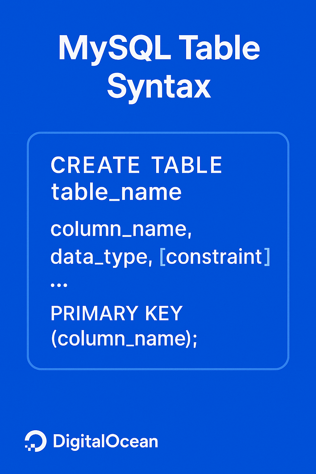
The syntax for creating a table in MySQL with a primary key is as follows:
CREATE TABLE table_name (
    column1_name data_type PRIMARY KEY,
    column2_name data_type,
    ...
);
A primary key is a column or set of columns in a table that uniquely identifies each row in the table. It ensures that no two rows have the same value(s) in the primary key column(s), which helps to maintain data integrity and prevent duplicate records. In the context of the example below, the
id column serves as the primary key, ensuring each user has a unique identifier.Example with Primary Key:
CREATE TABLE users (
    id INT PRIMARY KEY,
    name VARCHAR(255),
    email VARCHAR(255)
);
MySQL Table Syntax without Primary Key
The syntax for creating a table in MySQL without a primary key is as follows:CREATE TABLE table_name (
column1_name data_type,
column2_name data_type,
...
);
Most Common MySQL Commands Table
Here’s a table summarizing the MySQL commands used in this tutorial, including their syntax, usage, and examples:| Command | Syntax | Description | Example |
|---|---|---|---|
CREATE DATABASE |
CREATE DATABASE database_name; |
Creates a new database | CREATE DATABASE mydatabase; |
USE |
USE database_name; |
Selects the database to use for the current session | USE mydatabase; |
CREATE TABLE |
CREATE TABLE table_name (column1_name data_type, column2_name data_type, ...); |
Creates a new table in the database | CREATE TABLE users (id INT PRIMARY KEY, name VARCHAR(255), email VARCHAR(255)); |
INSERT INTO |
INSERT INTO table_name (column1_name, column2_name, ...) VALUES (value1, value2, ...); |
Inserts new records into a table | INSERT INTO users (name, email) VALUES ('John Doe', '<john@example.com>'); |
SELECT |
SELECT column1_name, column2_name, ... FROM table_name; |
Retrieves data from a database table | SELECT * FROM users; |
UPDATE |
UPDATE table_name SET column1_name = value1, column2_name = value2, ... WHERE condition; |
Updates existing records in a table | UPDATE users SET name = 'Jane Doe' WHERE id = 1; |
REPLACE |
REPLACE INTO table_name (column1_name, column2_name, ...) VALUES (value1, value2, ...); |
Inserts new records into a table, or replaces existing records if a unique key constraint is violated | REPLACE INTO users (id, name, email) VALUES (1, 'Jane Doe', 'jane.doe@example.com'); |
DROP TABLE |
DROP TABLE IF EXISTS table_name; |
Deletes a table from the database | DROP TABLE IF EXISTS users; |
DROP DATABASE |
DROP DATABASE IF EXISTS database_name; |
Deletes a database | DROP DATABASE IF EXISTS mydatabase; |
Step 1 - Create a Database
To begin, you need to create a new database where your table will be stored. This is done using the CREATE DATABASE statement, followed by the name of the database you want to create. In this example, we’re creating a database named mydatabase.CREATE DATABASE mydatabase;
USE statement. This ensures that any subsequent operations are performed within the context of the newly created database.USE mydatabase;
Step 2 - Create a Table
To create a table in MySQL, you use the CREATE TABLE statement followed by the name of the table you want to create. In this example, we’re creating a table named users. The table definition is enclosed in parentheses and consists of four columns: id, name, email, and registration_date.Here’s a breakdown of each column:
CREATE TABLE users (
    id INT PRIMARY KEY AUTO_INCREMENT,
    name VARCHAR(100),
    email VARCHAR(255) UNIQUE,
    registration_date DATE
);
-
id: This column is defined as an integer (INT) and is set as the primary key of the table usingPRIMARY KEY. TheAUTO_INCREMENTattribute means that each time a new record is inserted into the table, the value ofidwill automatically increase by 1, starting from 1. This ensures that each record has a unique identifier.
-
nameandemail: These columns are defined as variable-length strings usingVARCHAR. The number in parentheses specifies the maximum length of the string that can be stored in each column. Forname, the maximum length is 100 characters, and foremail, it’s 255 characters. TheUNIQUEattribute foremailensures that each email address in the table is unique and cannot be duplicated.
-
registration_date: This column is defined as aDATEtype, which is used to store dates. It will hold the date when each user registered.
CREATE TABLE statement, you have successfully created a new table named users with the specified columns and their properties.
Step 3 - Insert Data into the Table
To insert data into the users table, you will use the INSERT INTO statement. This statement is followed by the table name, users, and the columns where you want to insert data, which are name, email, and registration_date. The VALUES keyword is then used to specify the actual values to be inserted into these columns.In this example, the values being inserted are:
name: ‘John Doe’email: ‘john@example.com’registration_date: ‘2025-01-10’
INSERT INTO users (name, email, registration_date)
VALUES ('John Doe', 'john@example.com', '2025-01-10');
users table with the specified values.Inserting Multiple Rows
When you need to insert multiple rows into a table, using a singleINSERT INTO statement with multiple VALUES clauses can be more efficient than executing separate INSERT INTO statements for each row. This approach reduces the number of database interactions, which can improve performance and reduce the load on the database server.Here’s an example of how to insert multiple rows into the
users table in a single statement:INSERT INTO users (name, email, registration_date)
VALUES
('Jane Smith', 'jane@example.com', '2025-01-11'),
('Emily Johnson', 'emily@example.com', '2025-01-12');
users table with a single INSERT INTO statement. The VALUES clause is repeated for each row, separated by commas. This approach allows you to insert multiple rows in a single operation, making it more efficient than executing separate INSERT INTO statements for each row.
Step 4 - Verify the Data
After inserting data into the users table, it’s essential to verify that the data has been successfully inserted and is accurate. This step ensures that the data is consistent with the expected output and helps in identifying any potential issues early on.To verify the data insertion, you can use the
SELECT statement to retrieve all the records from the users table. The SELECT * syntax retrieves all columns (*) from the specified table (users). This allows you to view the entire dataset and confirm that the expected data is present.Here’s the SQL statement to verify the data:
SELECT * FROM users;
Output+----+------------+-------------------+----------------+
| id | name       | email             | registration_date |
+----+------------+-------------------+----------------+
|  1 | John Doe   | john@example.com | 2025-01-10      |
|  2 | Jane Smith | jane@example.com | 2025-01-11      |
|  3 | Emily Johnson | emily@example.com | 2025-01-12      |
+----+------------+-------------------+----------------+
Step 5 - Update Data
Updating existing records in a database is a crucial operation that allows you to modify data that has already been inserted. This process is essential for maintaining data accuracy and consistency over time. In this step, we will demonstrate how to update a specific record in the users table using the UPDATE statement.To update existing records, use the
UPDATE statement followed by the table name, the SET clause to specify the column(s) to update, and the WHERE clause to specify the condition for which records to update. Here’s an example of how to update the email address of a user with id equal to 1:UPDATE users SET email = 'john.doe@example.com' WHERE id = 1;
UPDATE statement, it’s essential to verify that the data has been successfully updated. To do this, use the SELECT statement to retrieve the updated record(s). The SELECT * syntax retrieves all columns (*) from the specified table (users). This allows you to view the entire dataset and confirm that the expected data is present.Here’s the SQL statement to verify the update:
SELECT * FROM users;
id equal to 1 has been successfully updated:Output+----+------------+-------------------+----------------+
| id | name | email | registration_date |
+----+------------+-------------------+----------------+
| 1 | John Doe | john.doe@example.com | 2025-01-10 |
| 2 | Jane Smith | jane@example.com | 2025-01-11 |
| 3 | Emily Johnson | emily@example.com | 2025-01-12 |
+----+------------+-------------------+----------------+
Practical Usage
Inserting data for a blog, CRM, or e-commerce site
In the context of a blog, CRM (Customer Relationship Management), or e-commerce site, inserting data into a database is a crucial operation. For instance, when a user registers on a blog or e-commerce site, their information needs to be stored in a database for future reference. Similarly, in a CRM system, customer data is inserted into the database to manage interactions and relationships. This process is essential for building a robust and scalable backend infrastructure.Here’s an example of how to insert user registration data into a database using PHP and MySQL:
<?php
// Assuming $conn is a valid MySQL connection
if (isset($_POST['register'])) {
    $name = $_POST['name'];
    $email = $_POST['email'];
    $password = $_POST['password']; // Assuming password is hashed for security

    $query = "INSERT INTO users (name, email, password) VALUES (?, ?, ?)";
    $stmt = $conn->prepare($query);
    $stmt->bind_param("sss", $name, $email, $password);
    $stmt->execute();
    $stmt->close();
}
?>
Integration with backend workflows
The ability to insert data into a database seamlessly integrates with various backend workflows. For example, in a web application, user registration data is typically inserted into a database using server-side languages like PHP, Python, or Node.js. This data is then used to authenticate users, manage their profiles, and provide personalized experiences. In a CRM system, data insertion is critical for tracking customer interactions, managing sales pipelines, and generating insights for business growth.Here’s an example of how to insert customer interaction data into a database using Node.js and MySQL:
const mysql = require('mysql');

// Assuming db is a valid MySQL connection
const insertCustomerInteraction = (customerID, interactionType, interactionDate) => {
    const query = "INSERT INTO customer_interactions (customer_id, interaction_type, interaction_date) VALUES (?, ?, ?)";
    db.query(query, [customerID, interactionType, interactionDate], (error, results, fields) => {
        if (error) throw error;
        console.log('Customer interaction inserted successfully');
    });
};
Common errors
Table already exists
When attempting to create a table that already exists in the database, MySQL will throw an error. To avoid this, you can use theIF NOT EXISTS clause in your CREATE TABLE statement. Here’s an example:CREATE TABLE IF NOT EXISTS users (
id INT AUTO_INCREMENT PRIMARY KEY,
name VARCHAR(255) NOT NULL,
email VARCHAR(255) UNIQUE NOT NULL
);
Incorrect data types
Using incorrect data types for columns can lead to errors or unexpected behavior. For instance, trying to insert a string into an integer column will result in an error. Ensure that the data types of your columns match the type of data you’re inserting.Example of incorrect data type usage:
CREATE TABLE users (
    id INT AUTO_INCREMENT PRIMARY KEY,
    name VARCHAR(255) NOT NULL,
    email VARCHAR(255) UNIQUE NOT NULL,
    age VARCHAR(3) NOT NULL // Incorrect data type for age, should be INT
);

INSERT INTO users (name, email, age) VALUES ('John Doe', 'john.doe@example.com', 'twenty-five'); // This will result in an error due to incorrect data type for age
CREATE TABLE users (
    id INT AUTO_INCREMENT PRIMARY KEY,
    name VARCHAR(255) NOT NULL,
    email VARCHAR(255) UNIQUE NOT NULL,
    age INT NOT NULL // Correct data type for age
);

INSERT INTO users (name, email, age) VALUES ('John Doe', 'john.doe@example.com', 25); // Correct insertion with the right data type for age
Syntax errors
Syntax errors can occur due to incorrect SQL syntax, such as missing or mismatched parentheses, incorrect use of keywords, or incorrect column names. To avoid syntax errors, ensure that your SQL statements are correctly formatted and follow the MySQL syntax guidelines.Example of syntax error:
INSERT INTO users (name, email, age VALUES ('John Doe', 'john.doe@example.com', 25); // Missing closing parenthesis
INSERT INTO users (name, email, age) VALUES ('John Doe', 'john.doe@example.com', 25); // Correctly formatted SQL statement
Difference between INSERT, INSERT IGNORE, and REPLACE
When working with MySQL, it’s essential to understand the differences between INSERT, INSERT IGNORE, and REPLACEINSERT, INSERT IGNORE, and REPLACE statements. Each of these statements serves a unique purpose in managing data insertion into tables. Here’s a detailed explanation of each statement, along with examples and a comparison table at the end.INSERT
The standardINSERT statement inserts a new row into a table. If the row already exists, it will throw an error. This is the most common method of inserting data into a table.INSERT INTO users (name, email) VALUES ('John Doe', 'john.doe@example.com');
INSERT IGNORE
INSERT IGNORE is similar to INSERT, but it ignores the error if the row already exists. This can be useful when you want to insert a row only if it doesn’t already exist. If the row already exists, the statement will silently ignore the insertion attempt.INSERT IGNORE INTO users (name, email) VALUES ('John Doe', 'john.doe@example.com');
REPLACE
REPLACE works similarly to INSERT, but if the row already exists, it replaces the existing row with the new data. This statement is particularly useful when you need to update existing data or ensure that duplicate rows are not inserted.REPLACE INTO users (name, email) VALUES ('John Doe', 'john.doe@example.com');
Comparison Table
Here’s a comparison table to help you understand the key differences betweenINSERT, INSERT IGNORE, and REPLACE:| Statement | Behavior if Row Exists | Error Handling |
|---|---|---|
| INSERT | Throws an error | Raises an error |
| INSERT IGNORE | Ignores the insertion | Silently ignores the error |
| REPLACE | Replaces the existing row | Raises an error if the row does not exist |
- Use
INSERTwhen you want to ensure that a row is inserted only if it doesn’t already exist, and you want to handle errors explicitly. - Use
INSERT IGNOREwhen you want to insert a row only if it doesn’t already exist, and you don’t care about handling errors. - Use
REPLACEwhen you want to ensure that a row is inserted or updated if it already exists, and you want to handle errors explicitly.
How to use prepared statements
Prepared statements are a secure way to execute SQL statements with dynamic inputs, protecting against SQL injection attacks by separating code from data. In PHP, use mysqli or PDO to prepare and execute statements. Here’s a concise example using mysqli:<?php
// Prepare an SQL statement to insert a new user into the 'users' table
$stmt = $conn->prepare("INSERT INTO users (name, email) VALUES (?, ?)");
// Bind the parameters to the SQL statement, specifying the types of the variables
$stmt->bind_param("ss", $name, $email);
// Assign values to the variables
$name = 'Jane Doe';
$email = 'jane.doe@example.com';
// Execute the prepared statement
$stmt->execute();
// Close the prepared statement
$stmt->close();
?>
mysqli or PDO usage.
FAQs
1. Can I create a table without defining a primary key?
Yes, you can create a table without defining a primary key. However, it’s highly recommended to define a primary key for each table to ensure data integrity and facilitate efficient data retrieval. Here’s an example of creating a table without a primary key:CREATE TABLE users (
name VARCHAR(255),
email VARCHAR(255)
);
2. How do I insert multiple rows in one query?
You can insert multiple rows in one query using the following syntax:INSERT INTO users (name, email) VALUES ('John Doe', 'john.doe@example.com'), ('Jane Doe', 'jane.doe@example.com');
3. What’s the difference between CHAR and VARCHAR in MySQL?
CHAR and VARCHAR are both character data types in MySQL, but they differ in how they store and handle data.CHAR is a fixed-length string that always occupies the same space, padding with spaces if necessary. For example, CHAR(10) will always store 10 characters, even if the actual data is shorter.VARCHAR, on the other hand, is a variable-length string that only occupies the space needed to store the actual data. It’s more efficient for storing strings of varying lengths.Here’s an example of using both
CHAR and VARCHAR:CREATE TABLE users (
name CHAR(10),
email VARCHAR(255)
);
4. How do I copy and create a new table in MySQL?
You can copy and create a new table in MySQL using the following syntax:CREATE TABLE new_users SELECT * FROM users;
new_users with the same structure and data as the users table.5. How to create a database in MySQL?
To create a database in MySQL, use the following command:CREATE DATABASE mydatabase;
mydatabase.
Conclusion
In this tutorial, you have learned how to create and insert a table in MySQL using simple SQL commands. You have also covered some common errors and how to avoid them. This is just the beginning of your MySQL journey. To further enhance your skills, consider exploring these additional tutorials:- How to Create a New User and Grant Permissions in MySQL
- How to Use Indexes in MySQL
- How to Fix Corrupted Tables in MySQL
- How to Create and Manage Tables in SQL
The experiments were run on bare-metal H100 multi-node clusters, scaling from 1 to 8 nodes. Across all configurations, the infrastructure consistently delivered expected performance improvements as nodes increased, with efficient resource utilization across CPU, GPU, storage, and interconnect networking.
These results demonstrate that DigitalOcean’s infrastructure is optimized and production-ready for demanding AI workloads such as large-scale LLM training. This serves as a validation for customers looking to scale up without the operational burden of infrastructure tuning.
Introduction
This report provides a comprehensive analysis of the end-to-end efficacy and performance of pretraining and finetuning of large language models in a multinode setting. We use DO’s bare-metal infrastructure on 8 nodes.MosaicML LLM Foundry provides a framework in which multinode pretraining and finetuning is supported, including not only model finetuning, but verification of model inference functionality and model accuracy via evaluation, representing a true end-to-end system.
- Finetuning tool:
- MosaicML LLM Foundry
- Tasks:
- Full pretraining from scractch
- Finetuning of pretrained model
- Models:
- Pretraining
- MPT-125M, 350M, 760M, 1B, 3B, 7B, 13B, 30B, 70B
- Finetuning
- MPT-7B-Dolly-SFT
- MPT-30B-Instruct
- Pretraining
- Data:
- Pretraining
- C4
- Finetuning
- Dolly HH-RLHF
- Instruct-v3
- Pretraining
- Key metrics:
- Token throughput (tok/s)
- Model FLOPS uilization (MFU)
- Runtime (wallclock)
- Scenario dimensions:
- Pretraining
- Model sizes: 125M, 350M, 760M, 1B
- Finetuning
- Number of nodes: 1, 2, 4, 8
- Pretraining
For full details of the hardware, software, pretraining & finetuning datasets, and network speed tests, see the appendices.
Results and discussion
In this section, we examine the results of our full pretraining and finetuning experiments. We find that model pretraining and finetuning both run successfully on DO multinode bare-metal machines, and can be run by users.Full pretraining
Our full pretraining runs are shown in Table 1. We do not graph these due to the small number of rows and variety of relevant results encapsulated in the table.| Model | Training data | Max duration (batches) | Ratio params / 125M params | Ratio batches / 125M batches | Evaluation interval (batches) | No. nodes | Actual runtime (wallclock) | Actual runtime (s) | Ratio runtime / 125M runtime | Throughput (tokens/s) | Model FLOPS utilization (MFU) | Memory per GPU (from 82GB) | Checkpoint size | Conversion, inference & evaluation ok? | Evaluation accuracy |
|---|---|---|---|---|---|---|---|---|---|---|---|---|---|---|---|
| MPT-125M | C4 | 4800 | 1 | 1 | 1000 | 8 | 9m7.873s | 547.9 | 1 | 6,589,902 | ~0.1 | 13.4 | 1.5G | Y | 0.53 |
| MPT-350M | C4 | 13400 | 2.8 | 2.8 | 1000 | 8 | 38m10.823s | 2291 | 4.18 | 3,351,644 | ~0.145 | 8.91 | 4.0G | Y | 0.56 |
| MPT-760M | C4 | 29000 | 6.08 | 6.0 | 2000 | 8 | 103m23.136s | 6203 | 11.32 | 2,737,276 | ~0.27 | 12.5 | 8.6G | Y | 0.56 |
| MPT-1B | C4 | 24800 | 8 | 5.2 | 2000 | 8 | 208m24.319s | 12504 | 22.82 | 2,368,224 | ~0.33 | 16.3 | 15G | Y | 0.58 |
Main observations for full pretraining:
- In all cases, inference using the trained model, and model accuracy via evaluation on unseen testing data are verified.
- Model conversion after training to Hugging Face format, which gives a lighter weight model that is more efficient for inference, is also verified.
- The larger models in the MPT series, MPT-3B, -7B, -13B, -30B, and -70B, would run in the exact same way, but would require increasingly more wallclock time.
- Projection of runtime indicates that the largest model, MPT-70B, could be fully pretrained on DO in approximately 2 months on 8 nodes, or approximately 1 week on 64 nodes.
- Model FLOPS utilization, a measure of GPU usage more effective than raw utilization provided by LLM Foundry, is good, showing that the increased runtimes are genuine larger compute required by the larger models, not inefficiency of the infrastructure.
Finetuning
Similar to pretraining, we tabulate results for finetuning in Table 2.| Model | Finetuning data | Max training duration (epochs) | Evaluation Interval (epochs) | No. Nodes | Actual runtime (wallclock) | Actual runtime (s) | Speedup versus one node | Throughput (tokens/s) | Memory per GPU (from 82GB) | Inference & evaluation ok? | Evaluation accuracy |
|---|---|---|---|---|---|---|---|---|---|---|---|
| MPT-7B-Dolly-SFT | mosaicml/dolly_hhrlhf | 2 | 1 | 1 | 78m28.121s | 4708 | - | 7124 | 24.9 | Y | 0.85 |
| MPT-7B-Dolly-SFT | mosaicml/dolly_hhrlhf | 2 | 1 | 2 | 29m24.485s | 1764 | 2.67x | 13,844 | 19.9 | Y | 0.84 |
| MPT-7B-Dolly-SFT | mosaicml/dolly_hhrlhf | 2 | 1 | 4 | 18m21.026s | 1101 | 4.28x | 28,959 | 17.5 | Y | 0.84 |
| MPT-7B-Dolly-SFT | mosaicml/dolly_hhrlhf | 2 | 1 | 8 | 13m35.352s | 815 | 5.77x | 50,708 | 9.37 | Y | 0.84 |
| MPT-30B-Instruct | kowndinya23/instruct-v3 | 2 | 1 | 8 | 125m12.579s | 7513 | 3.76x | 52,022 | ~36 | Y | 0.85 |
Main observations for finetuning:
- The ideal speedup versus one node is N times for N nodes. We observe 2.67, 4.28, and 5.77x for 2, 4, and 8 nodes respectively. This indicates that we strongly gain from 2-4 nodes, a bit less so for 8. There is some overhead for model checkpoint saving after each epoch, but this is a normal operation.
- In all cases, inference using the trained model, and model accuracy via evaluation on unseen testing data are verified.
- Evaluation accuracy of the model on unseen data is higher than for the pretrained smaller models, as expected.
Appendices
Datasets for pretraining and finetuning
Pretraining dataset
For large language models, full pretraining from scratch requires a large generic dataset on which to train the model to give it basic language capabilities. MosaicML’s LLM Foundry provides support for the C4 dataset, which we used throughout pretraining.C4 is a standard text dataset for pretraining large language models, consisting of over 10 billion rows of data. It is a cleaned version of the Common Crawl web corpus. The data are downloaded and preprocessed as part of the end-to-end support of LLM Foundry for pretraining.
Finetuning dataset
Finetuning datasets are more specialized and smaller than pretraining datasets. We again used two examples supported by MosaicML, with some modifications for the 30B model.MPT-7B-Dolly-SFT
For finetuning the 7B model, we used the Dolly HH-RHLF dataset.From the dataset card, “This dataset is a combination of Databrick’s dolly-15k dataset and a filtered subset of Anthropic’s HH-RLHF. It also includes a test split, which was missing in the original dolly set. That test set is composed of 200 randomly selected samples from dolly + 4,929 of the test set samples from HH-RLHF which made it through the filtering process. The train set contains 59,310 samples; 15,014 - 200 = 14,814 from Dolly, and the remaining 44,496 from HH-RLHF.”
MPT-30B-Instruct
For finetuning the 30B model, we used the Instruct-v3 dataset, which consists of prompts and responses for instruction finetuning. The original MosaicML location contained a bug in which the dataset had incorrect columns, so we used a copy at kowndinya23/instruct-v3 where the relevant correction had been made. This was preferable to manually correcting because by default the end-to-end process points to remote dataset locations such as Hugging Face.Network Speed: NCCL Tests
NCCL tests were run on the machines used for this project, verifying the efficacy of the network.Our purpose was simple hardware verification, and more extensive testing has been carried out elsewhere by DO infrastructure teams. However, these results have been of interest as an available representation of our typical networking speeds by customers interested in multinode work, so we supply them here.
This command was used to generate the results:
mpirun \
-H hostfile \
-np 128 \
-N 8 \
--allow-run-as-root \
-x NCCL_IB_PCI_RELAXED_ORDERING=1 \
-x NCCL_IB_CUDA_SUPPORT=1 \
-x NCCL_IB_HCA^=mlx5_1,mlx5_2,mlx5_7,mlx5_8 \
-x NCCL_CROSS_NIC=0 -x NCCL_IB_GID_INDEX=1 \
$(pwd)/nccl-tests/build/all_reduce_perf -b 8 -e 8G -f 2 -g 1
| Size (B) | Count (elements) | Type | Redop | Root | Out-of-place | In-place | ||||||
|---|---|---|---|---|---|---|---|---|---|---|---|---|
| Time (us) | Algbw (GB/s) | Busbw (GB/s) | #Wrong | Time (us) | Algbw (GB/s) | Busbw (GB/s) | #Wrong | |||||
| 8 | 2 | float | sum | -1 | 63.25 | 0.00 | 0.00 | 0 | 65.28 | 0.00 | 0.00 | 0 |
| 16 | 4 | float | sum | -1 | 63.10 | 0.00 | 0.00 | 0 | 62.37 | 0.00 | 0.00 | 0 |
| 32 | 8 | float | sum | -1 | 62.90 | 0.00 | 0.00 | 0 | 63.54 | 0.00 | 0.00 | 0 |
| 64 | 16 | float | sum | -1 | 63.23 | 0.00 | 0.00 | 0 | 63.40 | 0.00 | 0.00 | 0 |
| 128 | 32 | float | sum | -1 | 64.08 | 0.00 | 0.00 | 0 | 63.23 | 0.00 | 0.00 | 0 |
| 256 | 64 | float | sum | -1 | 63.81 | 0.00 | 0.01 | 0 | 63.33 | 0.00 | 0.01 | 0 |
| 512 | 128 | float | sum | -1 | 67.62 | 0.01 | 0.02 | 0 | 66.06 | 0.01 | 0.02 | 0 |
| 1024 | 256 | float | sum | -1 | 71.55 | 0.01 | 0.03 | 0 | 70.99 | 0.01 | 0.03 | 0 |
| 2048 | 512 | float | sum | -1 | 76.07 | 0.03 | 0.05 | 0 | 74.32 | 0.03 | 0.05 | 0 |
| 4096 | 1024 | float | sum | -1 | 75.73 | 0.05 | 0.11 | 0 | 76.28 | 0.05 | 0.11 | 0 |
| 8192 | 2048 | float | sum | -1 | 77.84 | 0.11 | 0.21 | 0 | 75.27 | 0.11 | 0.22 | 0 |
| 16384 | 4096 | float | sum | -1 | 78.70 | 0.21 | 0.41 | 0 | 75.98 | 0.22 | 0.43 | 0 |
| 32768 | 8192 | float | sum | -1 | 81.08 | 0.40 | 0.80 | 0 | 76.56 | 0.43 | 0.85 | 0 |
| 65536 | 16384 | float | sum | -1 | 80.14 | 0.82 | 1.62 | 0 | 77.50 | 0.85 | 1.68 | 0 |
| 131072 | 32768 | float | sum | -1 | 91.96 | 1.43 | 2.83 | 0 | 95.47 | 1.37 | 2.72 | 0 |
| 262144 | 65536 | float | sum | -1 | 108.5 | 2.42 | 4.79 | 0 | 106.5 | 2.46 | 4.88 | 0 |
| 524288 | 131072 | float | sum | -1 | 113.9 | 4.60 | 9.13 | 0 | 113.6 | 4.62 | 9.16 | 0 |
| 1048576 | 262144 | float | sum | -1 | 122.6 | 8.55 | 16.97 | 0 | 121.3 | 8.64 | 17.15 | 0 |
| 2097152 | 524288 | float | sum | -1 | 140.5 | 14.92 | 29.61 | 0 | 140.8 | 14.89 | 29.55 | 0 |
| 4194304 | 1048576 | float | sum | -1 | 179.8 | 23.33 | 46.29 | 0 | 178.8 | 23.45 | 46.54 | 0 |
| 8388608 | 2097152 | float | sum | -1 | 241.4 | 34.75 | 68.96 | 0 | 239.9 | 34.96 | 69.38 | 0 |
| 16777216 | 4194304 | float | sum | -1 | 343.9 | 48.78 | 96.80 | 0 | 343.0 | 48.92 | 97.07 | 0 |
| 33554432 | 8388608 | float | sum | -1 | 548.5 | 61.18 | 121.40 | 0 | 550.1 | 61.00 | 121.04 | 0 |
| 67108864 | 16777216 | float | sum | -1 | 943.5 | 71.13 | 141.15 | 0 | 940.8 | 71.33 | 141.55 | 0 |
| 134217728 | 33554432 | float | sum | -1 | 1490.7 | 90.04 | 178.67 | 0 | 1489.5 | 90.11 | 178.81 | 0 |
| 268435456 | 67108864 | float | sum | -1 | 2547.9 | 105.36 | 209.07 | 0 | 2549.8 | 105.28 | 208.91 | 0 |
| 536870912 | 134217728 | float | sum | -1 | 4241.8 | 126.57 | 251.16 | 0 | 4248.9 | 126.35 | 250.73 | 0 |
| 1073741824 | 268435456 | float | sum | -1 | 6753.1 | 159.00 | 315.52 | 0 | 6739.1 | 159.33 | 316.17 | 0 |
| 2147483648 | 536870912 | float | sum | -1 | 12466 | 172.26 | 341.83 | 0 | 12383 | 173.43 | 344.14 | 0 |
| 4294967296 | 1073741824 | float | sum | -1 | 23774 | 180.65 | 358.49 | 0 | 23871 | 179.93 | 357.04 | 0 |
The same results are plotted in the figure, for bus bandwidth as a function of 1-8 nodes.

Figure: NCCL bus bandwidth test results for machines used in this report, for 1-8 nodes
Hardware and Software
DigitalOcean Bare-Metal machines
DO bare metal machines consisting of 8 H100x8 nodes and the nodes were linked by an RDMA over Converged Ethernet (RoCE) network with a common VPC, with a shared storage filesystem providing multiple terabytes of storage. Each node consisted of 8 H100 GPUs connected by NVLink, for a total of 64 GPUs. As bare-metal machines, the Ubuntu operating system was provided, and MosaicML was then run from a Docker container.As a consequence of MosaicML’s usage of shared drives without requiring SLURM, Docker containers had to be duplicated on each node, but once done funetuning runs can be executed using a single command on each node.
The shared nature of the machines resulted in 8 of the 16 nodes being used for this project.
MosaicML LLM Foundry
This is an open source tool that allows pretraining and finetuning of models in a multinode setting. Particular positive attributes of this tool are:- Emphasis on end-to-end usage, including data preparation, model training/finetuning, inference, and evaluation, like in real customer use cases.
- Command-line based interface that allows pretraining and finetuning to be instantiated in this setting without the requirement to write a lot of code specialized to a particular application.
- Shared disk multinode setup that avoided the need for setting up and usage of SLURM, unlike most multinode tools that introduce this complex additional overhead taken from the HPC world.
- Proof of efficient usage of GPU compute via the model FLOPS utilization (MFU) metric
- Existing benchmarks from MosaicML enabling calibration of expectations (e.g., of MFU), albeit on different machines so not 1:1 comparable with our numbers
- Support of real-world large language models in the MPT series
- Weights & Biases logging integration
We will provide multiple model tuning methods, including one-at-a-time tuning, manual grid search, and random search techniques. We will also provide Python code examples that demonstrate learning rate tuning techniques and performance evaluation methods.
Prerequisites
- Confidently write and run Python scripts while managing library installations.
- Practical experience with scikit-learn for training and evaluating machine learning models such as SVC and GradientBoostingClassifier.
- Understanding the distinction between model parameters and hyperparameters, training/validation/test sets, and evaluation metrics like accuracy, F1-score, and AUC.
- A Python environment where numpy, pandas, matplotlib, and scikit-learn libraries are installed.
- Comfort with concepts like bias-variance trade-off, loss functions, and gradient-based optimization.
Model Parameters vs. Hyperparameters
Model parameters represent the internal weights or coefficients that a machine learning model learns from data during training. These directly influence predictions (e.g., the prediction of a neural network depends on its learned weights).On the other hand, model hyperparameters represent external configurations that users manually set to direct the machine learning training. They remain constant throughout training because they guide the learning process instead of being learned from the data.
Why Tune Hyperparameters Manually?
Current machine learning libraries provide automated hyperparameter tuning capabilities. However, manual hyperparameter tuning can be useful in some specific situations. Let’s consider some of them:
Small Datasets or Simple Models
When dealing with small problems or basic algorithms, manual hyperparameter tuning can be the fastest approach. Automated methods may be overkill. Manually tuning parameters can be useful for small datasets or basic models, despite being time-intensive.
Resource Constraints
Automated hyperparameter search requires extensive computational power because it tries many possible combinations. Selective manual exploration of a few settings enables the development of an adequate model when resources are limited.
Expert Intuition
Practitioners with experience often have intuition about which hyperparameter ranges work well based on theoretical insights or previous experience. Using intuition to search hyperparameter values manually can achieve better solutions more quickly compared to automated blind searches.
Manual Hyperparameter Tuning for SVM: A Step-by-Step Guide
Let’s consider a binary classification problem (e.g., classifying tumors as benign vs malignant). We will use the scikit-learn Breast Cancer Wisconsin dataset for our analysis. We will also implement a support vector machine classifier using its default configuration settings.Establish a Baseline Model
Start by training a baseline model using the default hyperparameters. A baseline model allows you to establish a reference point by showing basic performance statistics upon which to improve. Let’s consider the following code:from sklearn.datasets import load_breast_cancer
from sklearn.model_selection import train_test_split
from sklearn.svm import SVC
from sklearn.metrics import accuracy_score, f1_score, roc_auc_score
# Load dataset and split into train/validation sets
X, y = load_breast_cancer(return_X_y=True)
X_train, X_val, y_train, y_val = train_test_split(
X, y, test_size=0.2, random_state=42, stratify=y
)
# Train a baseline SVM model with default hyperparameters
model = SVC(kernel='rbf', probability=True, random_state=42)
model.fit(X_train, y_train)
y_pred = model.predict(X_val)
# Evaluate baseline performance
print("Baseline accuracy:", accuracy_score(y_val, y_pred))
print("Baseline F1-score:", f1_score(y_val, y_pred))
print("Baseline AUC:", roc_auc_score(y_val, model.predict_proba(X_val)[:, 1]))
Baseline accuracy: 0.9298245614035088
Baseline F1-score: 0.9459459459459459
Baseline AUC: 0.9695767195767195
Why multiple metrics? Accuracy alone can be misleading, especially with imbalanced data. Our evaluation incorporates F1-score to balance precision/recall, along with AUC to rank performance over all classification thresholds. You can choose the metric that is aligned with your objective (such as F1 or AUC).
Choose Hyperparameters to Tune
Although models typically feature multiple settings, they are not equally important. The best practice is to focus initially on a limited number of key hyperparameters. For our SVM example, we will focus on two major hyperparameters, which are C and gamma.-
C (Regularization parameter): Controls the trade-off between model complexity and error on training data.
- Low C: The model applies stronger regularization, which can cause higher bias but reduce variance, increasing the risk of underfitting.
- High C: Weaker regularization, allowing the model to fit the training data more closely. This reduces bias but increases variance, increasing the risk of overfitting.
-
Gamma (Kernel coefficient): This determines how much influence a single training example has on the decision boundary.
- Low gamma: Points have broader influence, resulting in smoother, more generalized decision boundaries.
- High gamma: Each point impacts only its immediate neighborhood, which can lead to complex boundaries.
Tune Hyperparameters One-by-One (Manual Trial and Error)
You can adjust one key hyperparameter at a time to see how the model responds. Hyperparameter tuning can start with manual trial-and-error, which is the simplest tuning method.Procedure:
- Start your experiments by choosing a single hyperparameter to adjust (such as C in SVM models).
- Choose a series of candidate values for testing based either on intuition or default settings. Hyperparameters often show non-linear effects, which makes it beneficial to test C values on a logarithmic scale(e.g., 0.01, 0.1, 1, 10, 100).
- For each selected value, train the model and evaluate its performance on the validation set.
- Plot or print the results to determine the best value before choosing it as your starting point.
for C in [0.01, 0.1, 1, 10, 100]:
    model = SVC(kernel='rbf', C=C, probability=True, random_state=42)
    model.fit(X_train, y_train)
    val_ac = accuracy_score(y_val, model.predict(X_val))
    print(f"C = {C:<5} | Validation Accuracy = {val_ac:.3f}")
C = 0.01  | Validation Accuracy = 0.842
C = 0.1   | Validation Accuracy = 0.912
C = 1     | Validation Accuracy = 0.930
C = 10    | Validation Accuracy = 0.930
C = 100   | Validation Accuracy = 0.947
Moderate C (around 1) often achieves an effective balance between bias and variance.
Very high C (e.g., 100) may lead to minor overfitting, which sometimes increases accuracy but reduces generalization ability.
Next, you could fix C=1 and tune gamma similarly:
for gamma in [1e-4, 1e-3, 1e-2, 0.1, 1]:
    model = SVC(kernel='rbf', C=1, gamma=gamma, probability=True, random_state=42)
    model.fit(X_train, y_train)
    val_ac = accuracy_score(y_val, model.predict(X_val))
    print(f"gamma = {gamma:<6} | Validation Accuracy = {val_ac:.3f}")
gamma = 0.0001 | Validation Accuracy = 0.930
gamma = 0.001  | Validation Accuracy = 0.895
gamma = 0.01   | Validation Accuracy = 0.640
gamma = 0.1    | Validation Accuracy = 0.632
gamma = 1      | Validation Accuracy = 0.632
Key Takeaways
- Manual one-at-a-time tuning helps you to build intuition about hyperparameters’ effects.
- Use the validation set for hyperparameter selection and keep the test set for final evaluation to avoid overfitting.
- Using multiple evaluation metrics(Such as F1 and AUC) for robust evaluation can help to identify overfitting and bias/variance issues at early stages.
Manual Grid Search (Systematic Exploration)
After performing initial one-by-one explorations, a manual grid search will allow you to explore combinations of hyperparameters. The grid search approach involves setting up a grid of potential values for each hyperparameter before evaluating each combination against the model. Our approach included sweeping C over 0.1, 1, 10, 50, and γ ranged between 1e−4, 1e−3, 0.01, 0.1 as we trained an RBF-kernel SVM for each pair combination. We then evaluate their performance using the validation set. The combination of (C, γ) parameters that produces the highest validation accuracy was selected as our best_params while also tracking F1/AUC.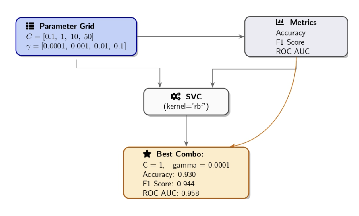
from sklearn.metrics import accuracy_score, f1_score, roc_auc_score

param_grid = {
    "C":     [0.1, 1, 10, 50],
    "gamma": [1e-4, 1e-3, 0.01, 0.1]
}

best_ac = 0.0
best_f1  = 0.0
best_auc = 0.0
best_params = {}

for C in param_grid["C"]:
    for gamma in param_grid["gamma"]:
        model = SVC(kernel='rbf',
                    C=C,
                    gamma=gamma,
                    probability=True,
                    random_state=42)
        model.fit(X_train, y_train)

        # Predictions and probabilities
        y_v_pred  = model.predict(X_val)
        y_v_proba = model.predict_proba(X_val)[:, 1]

        # metrics computation
        ac = accuracy_score(y_val, y_v_pred)
        f1  = f1_score(y_val, y_v_pred)
        auc = roc_auc_score(y_val, y_v_proba)

        # You can Track best by accuracy or change to f1/auc as needed
        if ac > best_ac:
            best_ac    = ac
            best_f1     = f1
            best_auc    = auc
            best_params = {"C": C, "gamma": gamma}

        print(f"C={C:<4}  gamma={gamma:<6}  => "
              f"Accuracy={ac:.3f}  F1={f1:.3f}  AUC={auc:.3f}")

print(
    "\nBest combo:", best_params,
    f"with Accuracy={best_ac:.3f}, F1={best_f1:.3f}, AUC={best_auc:.3f}"
)
Best combo: {'C': 1, 'gamma': 0.0001} with Accuracy=0.930, F1=0.944, AUC=0.958
Key points for manual grid search:
- The granularity of the grid matters. A coarse grid (few values) may overlook the best possible solution. A fine grid with numerous values increases the possibility of finding the best combination, but requires more training runs.
- When dealing with a large grid, it’s beneficial to apply cross-validation for a robust evaluation of each combination, but be aware that it increases computational requirements.
- Grid search suffers from the curse of dimensionality: Increasing hyperparameters or values can explode the number of combinations. At this point, random search emerges as a valuable strategy.
Manual Random Search for Hyperparameter Optimization
Start manual random search by selecting reasonable ranges for each hyperparameter. You can then randomly choose values within those ranges for several trials. In our experiment, we select C values from a log-uniform distribution between 0.1 and 100, and gamma values are selected between 1e-5 and 1e-2.The function below will enable you to conduct a random search across multiple metrics. It will allow you to identify optimal hyperparameters for Accuracy, F1-Score, and ROC AUC in one pass.

import random
import numpy as np
from sklearn.svm import SVC
from sklearn.metrics import accuracy_score, f1_score, roc_auc_score

def random_search_svm(X_train, y_train, X_val, y_val, ntrials=10):
    """
    Run random search across C and gamma parameters for an RBF SVM model.
    Monitor optimal hyperparameters for peak Accuracy, F1-score, and ROC AUC values.
    """
    best = {
        'accuracy': {'score': 0, 'params': {}},
        'f1':       {'score': 0, 'params': {}},
        'auc':      {'score': 0, 'params': {}}
    }

    for i in range(1, ntrials + 1):
        # Log-uniform sampling
        C = 10 ** random.uniform(-1, 2)       # 0.1 to 100
        gamma = 10 ** random.uniform(-5, -2)  # 1e-5 to 1e-2

        # model training
        model = SVC(kernel='rbf', C=C, gamma=gamma,
                    probability=True, random_state=42)
        model.fit(X_train, y_train)

        # Prediction and evaluation
        y_pred = model.predict(X_val)
        y_proba = model.predict_proba(X_val)[:, 1]
        ac = accuracy_score(y_val, y_pred)
        f1 = f1_score(y_val, y_pred)
        auc = roc_auc_score(y_val, y_proba)

        # Print trial results
        print(f"Trial {i}: C={C:.4f}, gamma={gamma:.5f} | "
              f"Acc={ac:.3f}, F1={f1:.3f}, AUC={auc:.3f}")

        # For each metric, we will update the best
        if ac > best['accuracy']['score']:
            best['accuracy'].update({'score': ac, 'params': {'C': C, 'gamma': gamma}})
        if f1 > best['f1']['score']:
            best['f1'].update({'score': f1, 'params': {'C': C, 'gamma': gamma}})
        if auc > best['auc']['score']:
            best['auc'].update({'score': auc, 'params': {'C': C, 'gamma': gamma}})

    # For each metric, print summary of best hyperparameters
    print("\nBest hyperparameters by metric:")
    for metric, info in best.items():
        params = info['params']
        score = info['score']
        print(f"- {metric.capitalize()}: Score={score:.3f}, Params= C={params.get('C'):.4f}, gamma={params.get('gamma'):.5f}")
Best hyperparameters by metric:
- Accuracy: Score=0.939, Params= C=67.2419, gamma=0.00007
- F1: Score=0.951, Params= C=59.5889, gamma=0.00002
- Auc: Score=0.987, Params= C=59.5889, gamma=0.00002
Evaluate Model Performance and Select the Best Model
Our validation set results show that the default RBF-SVM achieved strong baseline performance with 0.9298 accuracy, 0.9459 F1 score, and 0.9696 AUC.Testing all combinations of C values {0.1, 1, 10, 50} with γ values {1e-4, 1e-3, 0.01, 0.1} improved the accuracy by a small margin to reach 0.9300. The coarse grid search resulted in a lower AUC of 0.9580 and F1 score of 0.9440, indicating that it may have overlooked the most suitable kernel.
In contrast, a targeted random sampling approach within ranges C ∈ [0.1, 100] and γ ∈ [1e-5, 1e-2] reveals three distinct optimal parameter settings:
- Accuracy‐optimized: C ≈ 67.24, γ ≈ 7 × 10⁻⁵ (Accuracy = 0.9390)
- F1‐optimized: C ≈ 59.59, γ ≈ 2 × 10⁻⁵ (F1 = 0.9510)
- AUC‐optimized: C ≈ 59.59, γ ≈ 2 × 10⁻⁵ (AUC = 0.9870)
Primary Objective:
- If the ultimate goal is overall correctness, choose the Accuracy-optimized model.
- Go for the F1-optimized model if balanced precision and recall matter.
- The AUC-optimized model should be selected if ranking performance across thresholds is your priority.
The code example demonstrates how to load and split the dataset and then merge training and validation partitions, refitting the model with optimal settings, and evaluating its performance on the test data using accuracy, F1-score, and ROC AUC metrics.
from sklearn.datasets import load_breast_cancer
from sklearn.model_selection import train_test_split
from sklearn.svm import SVC
from sklearn.metrics import accuracy_score, f1_score, roc_auc_score
import numpy as np

# 1. data loading and spliting into train+val vs. test
X, y = load_breast_cancer(return_X_y=True)
X_tem, X_test, y_tem, y_test = train_test_split(
    X, y, test_size=0.2, random_state=42, stratify=y
)

# 2.Spliting X_tem into training and validation sets. We want to reproduce the previous split
X_train, X_val, y_train, y_val = train_test_split(
    X_tem, y_tem, test_size=0.25, random_state=42, stratify=y_tem
)
# Note that 0.25 of 80% give us 20% validation, that matches our original 80/20 split

# 3. We merge train and validation data for our final testing
X_merged = np.vstack([X_train, X_val])
y_merged = np.hstack([y_train, y_val])

# 4. Retrain using our best hyperparameters
best_C = 59.5889      # replace with your chosen C
best_gamma = 2e-05    # replace with your chosen gamma

f_model = SVC(
    kernel='rbf',
    C=best_C,
    gamma=best_gamma,
    probability=True,
    random_state=42
)
f_model.fit(X_merged, y_merged)

# 5. Evaluate on hold-out test set
y_test_pred = f_model.predict(X_test)
y_test_proba = f_model.predict_proba(X_test)[:, 1]

test_ac = accuracy_score(y_test, y_test_pred)
test_f1 = f1_score(y_test, y_test_pred)
test_auc = roc_auc_score(y_test, y_test_proba)

print("Final model test accuracy:   ", test_ac)
print("Final model test F1-score:    ", test_f1)
print("Final model test ROC AUC:     ", test_auc)
Tuning the Learning Rate
The learning rate is a critical hyperparameter during neural network training. For illustration, let’s explore a Gradient Boosting Classifier as our model.from sklearn.ensemble import GradientBoostingClassifier
for lr in [0.001, 0.01, 0.1, 0.3, 0.7, 1.0]:
model = GradientBoostingClassifier(n_estimators=50, learning_rate=lr, random_state=42)
model.fit(X_train, y_train)
val_acc = accuracy_score(y_val, model.predict(X_val))
print(f"Learning rate {lr:.3f} => Validation Accuracy = {val_acc:.3f}")
Learning rate 0.001 => Validation Accuracy = 0.632
Learning rate 0.010 => Validation Accuracy = 0.939
Learning rate 0.100 => Validation Accuracy = 0.947
Learning rate 0.300 => Validation Accuracy = 0.956
Learning rate 0.700 => Validation Accuracy = 0.956
Learning rate 1.000 => Validation Accuracy = 0.965
Developers commonly assess learning rates through a logarithmic scale progression with values such as 0.0001, 0.001, 0.01, 0.1, and 1.0. After identifying a suitable order of magnitude, you can test with intermediate values (such as 0.05, 0.1, 0.2, 0.3) to refine your selection.
Adjusting Regularization and Other Hyperparameters
Many models have a regularization parameter that can be adjusted:- In regression/SVM, the C value or the regularization penalty (L1/L2 strength) represents a hyperparameter.
- Neural networks use dropout rate and L2 weight decay as regularization hyperparameters.
- Decision trees utilize max_depth or min_samples_leaf to reduce complexity through their regularization function.
Tips and best practices for manual hyperparameter tuning
Manual tuning can become overwhelming because of the number of choices and potential interactions. Incorporating these practices into your tuning process ensures that each experiment is purposeful, reproducible, and interpretable.| Best Practice | Description |
|---|---|
| Coarse-to-Fine Search | Begin with a wide, log-scale range (very low to very high). Identify the region with best performance, then “zoom in” with smaller increments around that region. |
| One Change at a Time | Vary only a single hyperparameter per experiment. This isolation makes it clear which parameter caused any observed performance change. |
| Keep a Log | Record each hyperparameter setting and its results (e.g., in a notebook or printed output). This prevents duplicate trials and helps spot trends over time. |
| Use Validation Effectively | Always evaluate on held-out data. If data is limited, apply k-fold cross-validation. This ensures improvements reflect true generalization rather than fitting noise. |
| Mind Interactions | After isolating individual effects, explore combinations (e.g., learning rate + batch size, number of trees + learning rate). Hyperparameters often interact, and the optimal pair may differ from the individual optima. |
| Don’t Tune Too Many at Once | Focus on 2–3 key hyperparameters, leaving less critical ones at default values. |
| Stop When Returns Diminish | Set a target improvement (e.g., +2% accuracy). If further trials yield only marginal gains, conclude manual tuning or switch to automated methods for finer optimization. |
Practical scenarios where manual tuning shines
Manual hyperparameter tuning provides obvious benefits in several practical situations.
Small datasets or quick experiments Small datasets allow for rapid model training processes. Running multiple manual experiments can be a viable option when working with small datasets.
Debugging and prototyping
When a model fails to perform properly, manual tuning of a single parameter can help diagnose issues. For example, if raising max_depth fails to improve validation accuracy, it suggests that the problem may not be related to model complexity but rather the data quality.
Educational and Intuitive Understanding Manual hyperparameter tuning forces you to grasp the effects of each configuration on model behavior. This is great for learning and debugging. Understanding the bias-variance tradeoff becomes clearer as you observe how model behavior changes through increased complexity or added constraints.
When automated tuning fails
Automated searches often fail to escape suboptimal regions and may become confused by noise. Human intuition can spot patterns within results and choose to experiment with new approaches (for example, “all high values of parameter X perform poorly, so we will try a very low value of X”).
FAQ SECTION
Why manually tune ML parameters instead of using automation?
Using manual control methods develops intuition, saves computing resources, and resolves issues faster than black-box search techniques.What parameters should I tune first in a model? Focus tuning efforts on those hyperparameters that have the greatest impact on your model’s performance:
- When using neural networks, the learning rate is usually the primary hyperparameter to tune. Subsequently, you can tune the number of layers/units, batch size, and regularization strength, which includes L2 and dropout parameters.
- With tree-based models, tree depth, the number of trees (estimators), and the learning rate (for boosted trees) are important.
- For the SVM algorithm, the parameters C and kernel gamma, when using the RBF kernel.
- For k-Nearest Neighbors, the number of neighbors is k.
A model can benefit from manual tuning, particularly when the initial hyperparameters were poorly chosen. The default settings on many models lead to suboptimal performance for specific problems. Through manual tuning, you can elevate the accuracy levels of your model.
Is manual parameter tuning still relevant today? Absolutely. In the modern AutoML era, practitioners still depend on manual sweeps to meet performance, latency, and regulatory standards.
Conclusion
Data scientists and machine learning engineers must maintain manual hyperparameter tuning as a fundamental skill in their toolbox. Exploring various settings through one-at-a-time tests, manual grid searches, or random searches provides a comprehensive understanding of how key parameters influence the bias-variance trade-off and the model’s performance.Using best practices like coarse-to-fine searches, clear logging, and thorough validation makes each trial purposeful and reproducible. When running experiments on DigitalOcean GPU Droplets, you have full control over your compute environment—ideal for manually tweaking hyperparameters using frameworks like PyTorch or TensorFlow.
The manual approach lets you identify issues and teach concepts while making informed decisions when resources or time are limited.
For more in-depth tutorials and examples, explore these resources:
Introduction
Anyone who’s spent time generating images knows just how finicky image generation models can be about prompts. You’ll write what you think is a reasonable description, but the generated image doesn’t always match your vision. Even asking an LLM to refine your prompt gives you a verbose paragraph that sometimes does the trick. As a result, improving the quality of instruction-based image editing - that is, enhancing the model’s ability to adhere to prompts, is an active area of research.
Prerequisites
The goal of this tutorial is to give readers both an overview and implementation details of In-Context Edit (ICEdit), a technique that seeks to ameliorate the performance of instruction-based image editing. Useful prerequisites may include some familiarity with using image-generation models as well as language model concepts such as zero-shot prompting. We will be using DigitalOcean GPU Droplets to launch the gradio interface to allow you to play around with an ICEdit implementation. Feel free to skip sections that aren’t of use to you.
In-Context Edit (ICEdit)
Instruction-based image editing allows users to modify images with natural language, but existing approaches typically trade off precision for efficiency. Finetuning-based approaches achieve accuracy but require thousands to millions of examples and heavy computation, whereas training-free methods, such as manipulating attention weights, avoid that cost but often misinterpret complex instructions. ICEdit seeks to bridge this gap by leveraging a large pretrained Diffusion Transformer (DiT) to handle both the source image and editing prompt in one unified process.
Overview of Key Innovations
The paper, “In-Context Edit: Enabling Instructional Image Editing with In-Context Generation in Large Scale Diffusion Transformer” introduces three key innovations that together yield state-of-the-art results with minimal training:In-Context Editing
In-context editing is described as formulating editing as a conditional generation task by feeding the source image and edit instruction simultaneously (a diptych-style prompt) to the DiT. This zero-shot approach requires no new network modules and already achieves instruction compliance through the model’s built-in contextual attention.LoRA-MoE Hybrid Tuning
A parameter-efficient fine-tuning scheme where low-rank adapter (LoRA) modules are arranged as a mixture-of-experts. Here, a small gating network dynamically routes each task to the appropriate expert. This is very efficient as it enables diverse edits to be learned from only 50K samples while tuning ∼1% of the model parameters.VLM-Guided Noise Selection
An inference-time trick that generates a few initial noise seeds, runs only a few diffusion steps on each, and uses a Vision Language Model (VLM) to pick the seed whose partial output best matches the instruction. This ensures the final denoising starts from a favorable seed, greatly improving output consistency and alignment with the command.We’re going to go into more detail for those interested. Skip to the implementation section if you’d like to play around with the model.
In-Context Editing via Diffusion Transformers
At the core of ICEdit is a diffusion transformer (DiT) model, specifically the FLUX.1 Fill DiT (12B parameters). DiTs combine diffusion model generation with transformer attention, so that image and text inputs can be jointly attended to. The authors formulate in-context edit prompts (IC prompts) that contain both the reference image and the text instruction side by side, which they compare to a “diptych.”

Here, the left half of the input is the source image (the “reference”), and the right half is initially masked or noisy. The edit instruction (e.g. “make him grab a basketball with his hands”) is encoded with a T5 text encoder and appended to this input. The DiT then treats the task as generation: it reconstructs the left image (ensuring identity consistency) and simultaneously fills in the right side according to the instruction.
This in-context method has two major benefits: (1) No architectural changes: it avoids adding separate “reference encoders” or extra modules, since the DiT’s self-attention inherently processes the image half as context. (2) Tuning-free compliance: even without any additional training, the DiT often correctly localizes and applies the edit. The paper shows that attention maps on the edit prompt focus on the target region, indicating the model interprets the instruction as part of the context. In other words, by framing editing as a conditional generation on a diptych input, the pretrained DiT can follow instructions out of the box.
LoRA-MoE Hybrid Fine-Tuning
To improve precision on difficult edits while maintaining efficiency, the researchers decided to incorporate a fine-tuning stage. They collect a compact editing dataset (~50K examples from MagicBrush and OmniEdit) and attach LoRA adapters to the DiT’s weights. LoRA inserts trainable low-rank matrices into the linear projections of the model, which can be tuned with only a fraction of the parameters. This step alone brings large gains: after LoRA tuning, the DiT better follows instructions and produces cleaner edits (e.g. consistently colouring or removing objects as directed). However, the authors note that different edit types require different transformations of the image features. A single LoRA solution (shared across all tasks) may not capture this diversity.To address this, ICEdit introduces a Mixture-of-Experts (MoE) scheme for the LoRA modules. Instead of one adapter per layer, they insert multiple parallel LoRA “experts” (each with its own weight matrices) into the output projection of the multimodal attention block. A small routing network, conditioned on the current visual tokens and text embedding, decides which expert(s) to activate for each input. In practice they use a sparse MoE: only the top-k scoring experts (often k=1) are applied for a given sample, keeping computation low.
This LoRA-MoE design offers two key advantages: specialization and dynamic routing.
Specialization: Each expert adapter can specialize in a subset of editing behaviours (e.g. one expert might learn colour/style changes, another learns object insertion, etc.)
Dynamic routing: For each new instruction-image pair, the router selects the expert best suited to that task. As a result, the model can adapt on-the-fly to diverse editing requests without manual task switching.
The total added parameters remain small. The paper uses 4 experts of rank 32 in the DiT, which is roughly 1% of the full model parameters.
Empirically, this hybrid tuning yields substantial improvements over a single LoRA.
Post-tuning, ICEdit achieves state-of-the-art edit success rates across benchmarks while still avoiding full-model retraining. In essence, LoRA-MoE augments the in-context editing mechanism with learned expertise: the DiT retains its original architecture and data-free inference, but its outputs are now fine-tuned for precision on a variety of editing subtasks. This co-design of LoRA and MoE resolves the capacity limitations of lightweight tuning, enabling the model to express richer edit transformations.
VLM-Guided Noise Selection at Inference
The authors observe that the initial noise seed can drastically affect the edit outcome during inference, and that some seeds lead to much more accurate edits than others. In particular, they find that whether an edit is “working” often becomes evident after just a few diffusion steps. In light of this, they propose an early filtering strategy: sample multiple candidate seeds, run only a few diffusion steps (e.g. 4–10) for each, and then use a VLM to score which partial result best matches the edit instruction. The winning seed is then fully denoised to T steps to produce the final image.In practice, ICEdit uses a large multimodal model (Qwen2.5-VL-72B - note the paper says Qwen-VL-72B, but we believe they omitted the 2.5 by accident) as the scorer. The selection is done by pairwise comparisons: start with seed 0’s K-step output and seed 1’s and have the VLM judge which is more in line with the instruction (via natural language prompts or embeddings). The winner is then compared to seed 2’s output, and so on, effectively performing a tournament to pick the best seed.
This VLM-guided approach ensures the final edit is aligned with the instruction. By eliminating poor seeds early, the model avoids wasting computation on bad trajectories and gains robustness against randomness.
Now that we’ve covered the approach, let’s dig into the implementation!
Implementation
Step 1 : Set up a GPU Droplet
Begin by setting up a DigitalOcean GPU Droplet, select AI/ML and choose the NVIDIA H100 option.
Step 2: Web Console
Once your GPU Droplet finishes loading, you’ll be able to open up the Web Console.web console
Step 3: Install Dependencies and Clone the ICEdit Repo
In the web console, copy and paste the following code snippet:apt install python3-pip python3.10-venv
git clone https://github.com/River-Zhang/ICEdit
Step 4: Navigate to the correct repository
cd ICEdit
Step 5: Install Requirements
pip3 install -r requirements.txt
pip3 install -U huggingface_hub
Step 6: Obtain Flux Model Access
Agree to the conditions for the FLUX model since it will be used in the gradio implementation.
Step 7: Obtain Hugging Face Access Token
The HuggingFace token can be obtained from the Hugging Face Access Token page. Note that you may need to create a Hugging Face account. Ensure the appropriate boxes are selected before generating your token.
Step 8: Login to Hugging Face
huggingface-cli login
Step 9: Launch the Gradio app
python3 scripts/gradio_demo.py --share

Performance
Let’s take a look at how this model performs.


Based on the generated images - what are your thoughts on the model’s performance? Comment below.
Closing Thoughts
ICEdit, or In-Context Edit, offers a novel approach to instruction-based image editing by leveraging the power of Diffusion Transformers and innovative techniques like LoRA-MoE hybrid tuning and VLM-guided noise selection. These advancements significantly improve the model’s ability to adhere to complex instructions, leading to higher quality and more consistent edit results without extensive retraining, showcasing a promising direction for future image editing tools. We hope the implementation on DigitalOcean GPU Droplets went smoothly and you got a chance to play with ICEdit.Android Weekly 是一份专注于 Android 技术生态的周刊,每周一更新。本周刊深入挖掘 Android 系统架构、性能优化、跨平台开发、AI 等领域的高质量技术内容,为开发者提供持续的知识更新与技术洞察。
订阅渠道:[微信公众号] | [知乎专栏] | [掘金] | [RSS]
技术文章
- 一文看懂 2025 Google IO,誓把一切“装”上 Gemini,谷歌眼镜 10 年逆袭归来: 2025 年 Google I/O 大会聚焦 Gemini 技术,展示了其全面融入谷歌生态的最新进展,包括升级的 AI 模型、生成工具、搜索功能和智能眼镜等,旨在将 AI 技术深度嵌入日常生活和工作场景。
- Dart 3.8 发布,新格式化,新语法支持: Dart 3.8 发布,带来了多项重要更新,包括新的格式化功能、Null-Aware Elements 语法支持、Web 热重载初体验以及 FFigen 和 JNIgen 的原生互操作性支持等。
- Android 16 版本调测新特性汇总: 这篇文章主要总结了 Android 16 版本中的一些新特性和调测工具,重点关注性能、可靠性及调试能力的提升。文章详细介绍了多个模块的改进和新增功能,包括 tracing_perfetto 接口、Bitmap 维测能力、Native 内存统计、动态插桩能力、性能分析工具等。
- 安卓渲染管线能耗优化之刷新率和分辨率: 安卓渲染管线能耗优化主要围绕刷新率和分辨率的调整展开。通过基于用户注意力原则和不同 UI 场景,优化刷新率和分辨率设置以降低功耗。
- Binder 原理(二)之 Java 层源码分析: 本文详细分析了 Android Binder 机制的 Java 层源码实现,包括 Binder 的分层结构、AIDL 生成过程、进程间通信的发送与接收逻辑,以及 Stub 和 Proxy 的具体实现方式。
- Binder 原理(三)之通信内核: 本文详细解析了 Android Binder 通信机制的原理,包括其核心概念、内存映射方式、通信流程、源码分层结构以及 AIDL 和 Binder 的关系。文章还对 Binder 的一次拷贝机制、跨进程通信的实现方法以及内核驱动源码进行了深入探讨。
- Binder 原理(四)之 IPC 通信框架:服务发现、查找、调用: 本文详细解析了 Android 系统中 Binder 跨进程通信框架的原理与实现,包括服务注册、服务发现、服务调用的流程,并通过手写 IPC 通信框架的方式,帮助读者深入理解 Binder 框架的工作机制。同时,文章还介绍了 Android 系统启动流程中与 ServiceManager 和 system_server 相关的内容,以及动态代理在跨进程服务调用中的应用。
- Google IO - Navigation 3 使用介绍: 这篇文章介绍了 Navigation 3 的背景、主要变化、使用方法及其自适应布局的特点,并提供了源码和示例代码,帮助开发者更高效地处理复杂的导航需求。
- 2025 Google I/O 大会开发者主旨演讲干货盘点: 2025 Google I/O 开发者大会展示了多项创新技术,包括 AI 驱动的开发工具、生成式 AI 应用、跨平台开发支持等,助力开发者提升效率与创造力。
- 2025 KMP 的现状和未来,选择 KMP 会有什么问题吗?: 本文探讨了 Kotlin Multiplatform(KMP)的现状与未来发展,分析了其在国内外企业中的应用场景、存在的问题以及新功能和工具的改进,同时对 KMP 的技术差异和适用性进行了详细讨论。
- 拯救你的日志系统!Android 日志打印实战指南: 这篇文章详细介绍了如何优化和提升 Android 日志系统的质量,从常见痛点到具体的实践指南,包括日志级别的合理使用、动态开关机制、统一日志格式、安全与隐私保护、性能优化策略以及日志安全处理流程等内容,同时推荐了多个优秀的开源日志库供开发者参考。
- Android V app 冷启动(12) 真窗显示: 本文详细分析了 Android V 应用冷启动过程中启动窗口的隐藏和移除机制,重点探讨了启动窗口 surface 和真窗 leash 的移除过程,并结合源码解读了相关动画的执行和完成流程。
- 探秘智能调度线程池-方案总览: 在电商行业中,传统固定参数线程池因无法适应动态业务场景而暴露出资源利用率低、响应速度衰减及稳定性隐患等问题。为解决这些瓶颈,文章提出了智能调度线程池的概念,通过引入机器学习预测模型动态调整线程池参数,从而提升资源利用率、优化性能并实现自适应业务场景。具体实现包括数据收集、模型训练、格式转换及动态调度等步骤,最终为电商 App 提供高效稳定的运行保障。
- 从 Google IO 看移动端发展: Google I/O 展示了移动端发展的新趋势,Jetpack Compose 生态持续升级,推出 Navigation 3 导航库、自适应布局和多项新特性,同时优化性能与稳定性,强化 CameraX 和 Media3 支持;Android Studio 增强了开发与调试工具;端侧 AI 通过 Gemma 模型及 MLkit、Firebase AI 套件加速发展,传统 XML 和 View 体系逐步退出,端侧 AI 和 AI 编程成为未来重点方向。
- Flutter 小技巧之:Flutter 3.32 的 Property Editor 生产力工具: Flutter Property Editor 是一个生产力工具,需要 Flutter 3.32+ 才能使用。它支持在 VS Code 和 Android Studio/IntelliJ 中通过可视化界面查看和修改 Widget 属性,结合 Flutter inspector 和热重载,开发者可以实时查看更改效果。该工具支持不同类型的属性输入和筛选功能,帮助开发者更高效地管理 Widget 的属性。
- Android 重修之路:Framework 开发之 AOSP 源码下载与编译: 这篇文章详细介绍了如何下载和编译 Android AOSP 源码,包括环境依赖、安装所需软件、下载源码以及编译 ROM 的具体步骤,并提供了一些实用的技巧和注意事项。
- 重学 input:为什么要进行二次拦截?interceptKeyBeforeQueueing 和 interceptKeyBeforeDispatching 区别: 该文章主要探讨了 Android 系统中两种关键的按键事件拦截方法:interceptKeyBeforeQueueing 和 interceptKeyBeforeDispatching,并详细分析了它们的触发阶段、应用场景及代码逻辑差异。文章还总结了这两种方法如何协同工作以确保系统快速响应全局操作,同时灵活处理应用层交互。
- 面试福利 2:安卓系统 Framework 开发面试题目汇总: 安卓系统 framework 开发面试题目汇总,文章主要整理了一些安卓 framework 开发相关的面试题目,涵盖了 socket 通信、Binder 机制、系统启动优化、性能分析等多个技术领域,并提供了部分解决思路或讨论方式,适合面试前准备和提升技术理解。
- Flutter 图片预加载: 本文详细介绍了一个名为 ImagePreloader 的 Flutter 图片预加载工具,支持批量并发加载、状态监听以及对 SVG 图片的兼容。文章从工具的主要功能、核心代码实现到使用示例,逐步讲解如何通过预加载优化用户体验。
- 吐槽一波车载应用开发恶心点: 这篇文章主要吐槽了 Android 车载应用开发中的复杂流程,尤其是车载 Launcher 应用的安装和启动问题,并提出了通过脚本优化流程的解决方案。
- Google I/O 2025:从研究到现实: 本文是关于 Google I/O 2025 大会上 Sundar Pichai 的讲话内容,介绍了 Google 在 AI 领域的最新进展、产品发布以及未来发展方向,涵盖了 Gemini 模型的迭代、AI 在搜索、通信、个性化服务等方面的应用,以及新技术如 Google Beam 和 Project Astra 的推出。
- Android 内存泄漏检测全解析:从手动分析到自动化治理的实战指南: 本文详细解析了 Android 内存泄漏的原理、常见场景、检测工具(手动与自动化),并结合代码示例介绍了如何定位和修复泄漏问题,同时分享了内存泄漏的预防与最佳实践。
- FART 主动调用组件设计和源码分析: 本文探讨了 Android 应用脱壳的现有问题,并详细分析了基于主动调用的自动化脱壳方法(FART)的设计与实现,包括主动调用链的构造、CodeItem 的提取与解析、以及如何实现对所有类和方法的主动加载与调用。
- FART 自动化脱壳框架简介与脱壳点的选择: 本文介绍了 FART 自动化脱壳框架的原理和实现,特别是在 ART 环境下如何通过主动调用实现 dex 文件的完整 dump 和函数修复。
杂记
- 谈国产手机谁能活下来?: 文章分析了国产手机市场的激烈竞争现状,指出低端市场价格战严重,厂商普遍面临亏损压力。华为和苹果凭借软硬件一体化及研发投入占据高端市场,小米通过 SOC 芯片量产展现研发潜力,VIVO 和 Oppo 则依靠稳定产品质量和特色调整逐步发展。荣耀虽有硬件创新优势,但缺乏品牌效应和营销突破,未来发展充满不确定性。整体来看,国产手机厂商需找到差异化定位才能在红海市场中生存。
- 陷入混沌,个人如何应对: 文章探讨了在混沌和不确定性中,个人如何通过构建人生系统、提前规划和资源储备来寻找确定性,同时强调投资和风险管理的重要性,以及以终为始的思维方式对实现时间自由和财务自由的帮助。
- 工作周年与 AI 焦虑:成长与挑战并存: 作者回顾了在 Folo 工作一年的经历,比以往工作都久,虽然曾因各种原因频繁换工作。一年来,他从零起步参与并主导了产品的设计、重构交互与功能,并快速完成了 Web 和 Mobile 的多端改造,团队仅 4 人,成就感十足。对未来仍有些焦虑,担心自身成长和产品前景,期待变得更好。同时,他表达了对 AI 迅速发展带来的焦虑:AI 虽然提升了生产效率,让非专业程序员也能做好开发,但让他担心自身能力退化,害怕成为可被替代的“低级程序员”。他感到在 AI 辅助下对新技术的自信提升,但也担忧不依赖 AI 时独立思考和编程能力的下降。
- 三十而砺 - 反思我的创业: 2025 年 5 月 21 日,作者回顾了四年创业的经历,尽管失败,但收获了宝贵的经验和成长。他反思了商业规律,强调了用户需求、推广和差异化价值的重要性,并分享了创业带来的认知升级和生活的动态平衡。未来计划转向定制项目和知识分享。
AI
- 从 Claude 4 发布和 Windsurf 并购案,看 AI 的终局: 从 Windsurf 被 OpenAI 以 30 亿美元收购的案例出发,文章探讨了 AI 行业的终局可能性,并分析了大模型对传统互联网流量生态的冲击、AI 创业者的机遇、以及中型企业在 AI 浪潮中的生存策略。文章还详细剖析了 Windsurf 的发展历程及其选择被收购的原因。
- Gemini 2.5:我们最智能的模型系列再升级: Gemini 2.5 是 Google 最新升级的智能模型系列,带来了显著的性能提升和新功能,包括更自然的对话体验、更高的安全性以及支持开发者使用的多种工具。2.5 Pro 和 2.5 Flash 在多个领域表现出色,并通过新的技术如 Deep Think 和文本转语音功能进一步增强了用户体验。
- 我们构建通用 AI 助手的愿景: 谷歌通过多模态基础模型 Gemini 2.5 Pro 和项目如 Project Astra、Project Mariner,致力于构建通用人工智能助手,具备多任务处理、视频理解、屏幕共享等能力,以提升生产力和生活质量,同时将 AI 安全与伦理作为核心指导,推动科学进步和技术创新。
鸡血

投稿指南
欢迎投稿分享您的:- 技术博客
- 实践经验
- 工具推荐
- 公众号后台回复”投稿”
- 本周刊下面留言
- 发邮件 :dreamtale.jg@gmail.com
- 微信联系:Gracker_Gao
关于作者
下面是个人的介绍和相关的链接,期望与同行的各位多多交流,三人行,则必有我师!- 掘金 - Gracker:https://juejin.cn/user/1816846860560749
- 知乎 - Gracker:https://www.zhihu.com/people/gracker
- 个人博客 - Android Performance : 写东西的地方
- 个人介绍 - 欢迎加微信群组多多交流 :里面有个人的微信和微信群链接。
- 个人整理和搜集的优秀博客文章 - Android 性能优化必知必会 :欢迎大家自荐和推荐 (微信私聊即可)
- 微信公众号 Android Performance :

- Android 性能优化知识星球 : 个人运营的一个知识星球,欢迎加入,多谢支持~

版权声明
- 本周刊遵循 CC BY-NC-SA 4.0 协议
- 转载请注明出处:Android Weekly 第 X 期
- 欢迎订阅、分享,让更多开发者受益